Advanced Machine Learning
17: Expectation Maximization
Schedule (you are here )
| # | date | topic | description |
|---|---|---|---|
| 1 | 25-Aug-2025 | Introduction | |
| 2 | 27-Aug-2025 | Foundations of learning | Drop/Add |
| 3 | 01-Sep-2025 | Labor Day Holiday | Holiday |
| 4 | 03-Sep-2025 | Linear algebra (self-recap) | HW1 |
| 5 | 08-Sep-2025 | PAC learnability | |
| 6 | 10-Sep-2025 | Linear learning models | |
| 7 | 15-Sep-2025 | Principal Component Analysis | Project ideas |
| 8 | 17-Sep-2025 | Curse of Dimensionality | |
| 9 | 22-Sep-2025 | Bayesian Decision Theory | HW2, HW1 due |
| 10 | 24-Sep-2025 | Parameter estimation: MLE | |
| 11 | 29-Sep-2025 | Parameter estimation: MAP & NB | finalize teams |
| 12 | 01-Oct-2025 | Logistic Regression | |
| 13 | 06-Oct-2025 | Kernel Density Estimation | |
| 14 | 08-Oct-2025 | Support Vector Machines | HW3, HW2 due |
| 15 | 13-Oct-2025 | * Midterm | Exam |
| 16 | 15-Oct-2025 | Matrix Factorization | |
| 17 | 20-Oct-2025 | * Mid-point projects checkpoint | * |
| 18 | 22-Oct-2025 | k-means clustering |
| # | date | topic | description |
|---|---|---|---|
| 19 | 27-Oct-2025 | Expectation Maximization | |
| 20 | 29-Oct-2025 | Stochastic Gradient Descent | HW4, HW3 due |
| 21 | 03-Nov-2025 | Automatic Differentiation | |
| 22 | 05-Nov-2025 | Nonlinear embedding approaches | |
| 23 | 10-Nov-2025 | Model comparison I | |
| 24 | 12-Nov-2025 | Model comparison II | HW5, HW4 due |
| 25 | 17-Nov-2025 | Model Calibration | |
| 26 | 19-Nov-2025 | Convolutional Neural Networks | |
| 27 | 24-Nov-2025 | Thanksgiving Break | Holiday |
| 28 | 26-Nov-2025 | Thanksgiving Break | Holiday |
| 29 | 01-Dec-2025 | Word Embedding | |
| 30 | 03-Dec-2025 | * Project Final Presentations | HW5 due, P |
| 31 | 08-Dec-2025 | Extra prep day | Classes End |
| 32 | 10-Dec-2025 | * Final Exam | Exam |
| 34 | 17-Dec-2025 | Project Reports | due |
| 35 | 19-Dec-2025 | Grades due 5 p.m. |
Outline for the lecture
- Do we even need EM for GMM?
- GMM estimation: a hack
- MLE via EM
Do we even need EM for GMM?
Gaussian Mixture Model
Likelihood: $ \sum_{k=1}^K \pi_k\prob{N}{\vec{x}|\vec{\mu}_k, \bm{\Sigma}_k} $
\begin{align} \mbox{ for simplicity }\bm{\Sigma}_k & = \sigma^2 \bm{I}\\ \prob{p}{\vec{x}|y=k} & = \prob{N}{\vec{\mu}_k, \sigma^2 \bm{I}}\\ \prob{p}{y=k} & = \pi_k\\ \mbox{parameters: } & \vec{\mu}_1, \dots \vec{\mu}_K, \\ &\sigma^2, \\ & \pi_1, \dots, \pi_K \end{align}
Maximum (Log) Likelihood Estimation
\begin{align} \ln{ \prob{p}{\bm{X}|\{\vec{\mu}_k\}, \{\bm{\Sigma}_k\}}} &= \sum_{n=1}^N\ln\{\sum_{k=1}^K \pi_k\prob{N}{\vec{x}_n|\vec{\mu}_k, \sigma_k\bm{I}} \} \end{align}
Difficult to optimize
- Remember the exponential family? \[ \prob{p}{\vec{x}|\vec{\eta}} = \prob{h}{\vec{x}}\prob{g}{\vec{\eta}}e^{\vec{\eta}^T\prob{u}{\vec{x}}} \]
- How easy the $\log$-likelihood was back then \begin{align} \log{\cal L} & = \sum \log \prob{p}{\vec{x}|\vec{\eta}}\\ & = \sum \log \prob{h}{\vec{x}} + \sum \log \prob{g}{\vec{\eta}} + \sum \vec{\eta}^T\prob{u}{\vec{x}} \end{align}
- But $\sum \prob{p}{\vec{x}|\vec{\eta}}$ is not in the exponential familly
- \begin{align} \ln{ \prob{p}{\bm{X}| \{\vec{\mu}\}, \{\bm{\Sigma}\}}} &= \sum_{n=1}^N\ln\{\sum_{k=1}^K \pi_k\prob{N}{\vec{x}_n|\vec{\mu}_k, \sigma_k\bm{I}} \} \end{align}
Another problem (common to MLE)
- Suppose $K = 2$
- Suppose one $\vec{\mu}_k = \vec{x}_i$
- What's going to happen with our MLE? \begin{align} {\cal N}(x | \mu, \sigma_k) &= \frac{1}{\sqrt{2\pi\sigma^2}} e^{-\frac{(x_i-\mu_k)^2}{2\sigma_k^2}} \end{align}
\begin{align} {\cal N}(x | \mu, \sigma_k) &= \frac{1}{\sqrt{2\pi}}\frac{1}{\sigma_k^2}\\ \sigma_k &\to 0 \end{align}
GMM estimation: a hack
Mixture of 2 Gaussians
- \begin{align} \prob{p}{x_n|\mu_1, \mu_2, \sigma} &= \sum_{k=1}^2 \pi_k\prob{N}{x_n|\mu_k, \sigma} \end{align}
- \begin{align} \prob{p}{x_n|\mu_1, \mu_2, \sigma} &= \sum_{k=1}^2 \pi_k\frac{1}{\sqrt{2\pi\sigma^2}}\exp{\left(-\frac{(x-\mu_k)^2}{2\sigma^2}\right)} \end{align}
- Let's assume $\pi_1 = \pi_2 = 1/2$ and packing parameters to $\vec{\theta} = \{\mu_1, \mu_2, \sigma\}$
Mixture of 2 Gaussians
assuming known $\mu_k$ and $\sigma$
\begin{align} \prob{P}{k=1|x_n,\vec{\theta}} & = \frac{1}{1 + \exp{\left[-(w_1x_n+w_0)\right]}}\\ \prob{P}{k=2|x_n,\vec{\theta}} & = \frac{1}{1 + \exp{\left[+(w_1x_n+w_0)\right]}} \end{align}recall logistic regression and softmax!
Mixture of 2 Gaussians
assuming known $\sigma$ but not $\mu_k$
- \begin{align} \prob{p}{x_n|\mu_1, \mu_2, \sigma} &= \sum_{k=1}^2 \pi_k\frac{1}{\sqrt{2\pi\sigma^2}}\exp{\left(-\frac{(x-\mu_k)^2}{2\sigma^2}\right)} \end{align}
- \begin{align} \prob{p}{\bm{X}|\mu_1, \mu_2, \sigma} &= \underset{n}{\prod} \prob{p}{x_n|\mu_1, \mu_2, \sigma} \end{align}
- As you'll show, log-likelihood derivative is \begin{align} \frac{\partial {\cal L}}{\partial \mu_k} &= \sum_n \prob{P}{k|x_n,\vec{\theta}} \frac{x-\mu_k}{\sigma^2} \end{align}
Mixture of 2 Gaussians
assuming known $\sigma$ but not $\mu_k$
- As you'll show, log-likelihood derivative is \begin{align} \frac{\partial {\cal L}}{\partial \mu_k} &= \sum_n \prob{P}{k|x_n,\vec{\theta}} \frac{x-\mu_k}{\sigma^2} \end{align}
- As you'll show next$^{*}$ \begin{align} \frac{\partial^2 {\cal L}}{\partial^2 \mu_k} &= -\sum_n \prob{P}{k|x_n,\vec{\theta}} \frac{1}{\sigma^2} \end{align}
Ignore $\frac{\partial}{\partial \mu_k}\prob{P}{k|x_n,\vec{\theta}}$
Mixture of 2 Gaussians
assuming known $\sigma$ but not $\mu_k$
Using the good old Newton-Raphson update: $\mu = \mu - \frac{\partial {\cal L}}{\partial \mu_k}/\frac{\partial^2 {\cal L}}{\partial^2 \mu_k}$
You will show \[ \mu_k = \frac{\sum_n \left(\prob{P}{k|x_n,\vec{\theta}} x_n\right)}{\sum_n \prob{P}{k|x_n,\vec{\theta}} } \]
Compare to soft k-means: Iterations
Update
- Re-estimate the $K$ cluster centers (aka the centroid or mean), by assuming the memberships found above are correct. \begin{align} \hat{\mu}_k &= \frac{\underset{n}{\sum}r_k^n \vec{x}_n}{R_k}\\ R_k &= \underset{n}{\sum} r_k^n \end{align}
GMMs and k-means
- responsibilities are posteriors over latents
- update is maximization of the likelihood
Both "hacky" approaches to solve a latent variable problem use the same general technique
Expectation Maximization: a meta-algorithm
too important to simply skim!
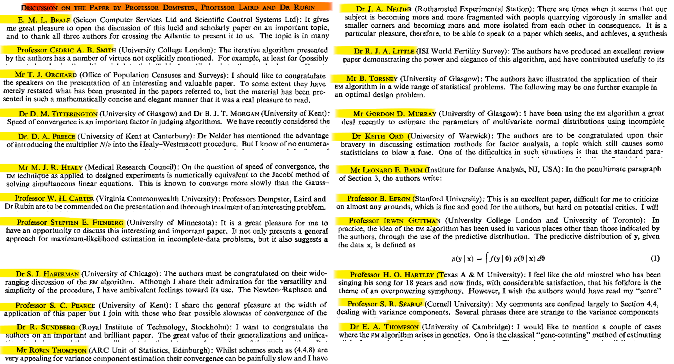
Convexity
Shades of Convex
Convex
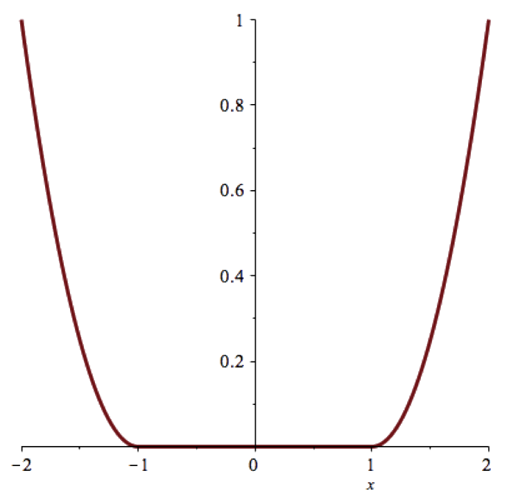
Strictly convex
Strongly convex
Convexity
Theorem:
if $f(x)$ is twice differentiable on $[a,b]$ and $f^{\prime \prime}(x) \ge 0$ on $[a,b]$ then $f(x)$ is convex on $[a,b]$.
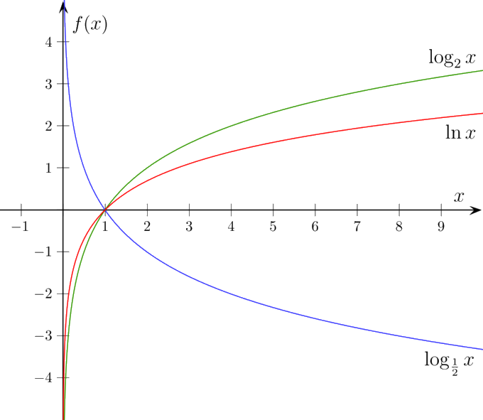
Convexity of logarithm
Theorem:
$-\ln(x)$ is strictly convex on $(0, \infty)$
Jensen's inequality
Theorem:
Let $f$ be a convex function on an interval $I$. If $x_1, x_2, \dots, x_n \in I$ with $\lambda_1, \lambda_2, \dots, \lambda_n \ge 0$ and $\sum_{i=1}^n\lambda_i=1$ \begin{align} f\left(\sum_{i=1}^n\lambda_ix_i\right) & \le \sum_{i=1}^n \lambda_i f(x_i) \end{align}
Thanks to Jensen's inequality
\begin{align} \ln\left(\sum_{i=1}^n\lambda_ix_i\right) & \le \sum_{i=1}^n \lambda_i \ln{(x_i)} \end{align}
Derivation of EM algorithm
- Our goal is to maximize the likelihood function: \[ \prob{L}{\vec{\theta}} = \ln \prob{P}{\bm{X}|\vec{\theta}} \]
- Equivalently if at step $n$ we have $\vec{\theta}_n$, we want such $\vec{\theta}$ \[ \prob{L}{\vec{\theta}} \gt \prob{L}{\vec{\theta}_n} \]
- Yet, equivalently we want to maximize \[ \prob{L}{\vth} - \prob{L}{\vec{\theta}_n} = \ln\prob{P}{\bm{X}|\vec{\theta}} - \ln\prob{P}{\bm{X}|\vec{\theta}_n} \]
-
Looks difficult!
Introducing random variables $\vec{z}$
- \[ \prob{P}{\bm{X}|\vec{\theta}} = \sum_{\vec{z}} \prob{P}{\bm{X}|\vec{z}, \vth}\prob{P}{\vec{z}|\vth} \]
- \[ \prob{L}{\vth} - \prob{L}{\vec{\theta}_n} = \ln\prob{P}{\bm{X}|\vec{\theta}} - \ln\prob{P}{\bm{X}|\vec{\theta}_n} \]
- Becomes \[ \prob{L}{\vth} - \prob{L}{\vec{\theta}_n} = \ln \sum_{\vec{z}} \prob{P}{\bm{X}|\vec{z}, \vth}\prob{P}{\vec{z}|\vth} - \ln\prob{P}{\bm{X}|\vec{\theta}_n} \]
Modifying the objective
Define the lower bound
\begin{align} {\cal L}(\vth|\vth_n) & \def \prob{L}{\vth_n} + \Delta(\vth|\vth_n)\\ \prob{L}{\vth} & \ge {\cal L}(\vth|\vth_n)\\ \end{align}When $\prob{L}{\vth} = {\cal L}(\vth|\vth_n)$
What happens when we optimize $\cal L$
What happens when we optimize $\cal L$
Kullback-Leibler divergence
