Advanced Machine Learning
14: Matrix Factorization
Outline for the lecture
- What are we talking about
- Independent Component Analysis
- Nonnegative Matrix Factorization
- Dictionary Learning
- Autoencoders
- Take home points
Schedule (you are here )
| # | date | topic | description |
|---|---|---|---|
| 1 | 25-Aug-2025 | Introduction | |
| 2 | 27-Aug-2025 | Foundations of learning | Drop/Add |
| 3 | 01-Sep-2025 | Labor Day Holiday | Holiday |
| 4 | 03-Sep-2025 | Linear algebra (self-recap) | HW1 |
| 5 | 08-Sep-2025 | PAC learnability | |
| 6 | 10-Sep-2025 | Linear learning models | |
| 7 | 15-Sep-2025 | Principal Component Analysis | Project ideas |
| 8 | 17-Sep-2025 | Curse of Dimensionality | |
| 9 | 22-Sep-2025 | Bayesian Decision Theory | HW2, HW1 due |
| 10 | 24-Sep-2025 | Parameter estimation: MLE | |
| 11 | 29-Sep-2025 | Parameter estimation: MAP & NB | finalize teams |
| 12 | 01-Oct-2025 | Logistic Regression | |
| 13 | 06-Oct-2025 | Kernel Density Estimation | |
| 14 | 08-Oct-2025 | Support Vector Machines | HW3, HW2 due |
| 15 | 13-Oct-2025 | * Midterm | Exam |
| 16 | 15-Oct-2025 | Matrix Factorization | |
| 17 | 20-Oct-2025 | * Mid-point projects checkpoint | * |
| 18 | 22-Oct-2025 | k-means clustering |
| # | date | topic | description |
|---|---|---|---|
| 19 | 27-Oct-2025 | Expectation Maximization | |
| 20 | 29-Oct-2025 | Stochastic Gradient Descent | HW4, HW3 due |
| 21 | 03-Nov-2025 | Automatic Differentiation | |
| 22 | 05-Nov-2025 | Nonlinear embedding approaches | |
| 23 | 10-Nov-2025 | Model comparison I | |
| 24 | 12-Nov-2025 | Model comparison II | HW5, HW4 due |
| 25 | 17-Nov-2025 | Model Calibration | |
| 26 | 19-Nov-2025 | Convolutional Neural Networks | |
| 27 | 24-Nov-2025 | Thanksgiving Break | Holiday |
| 28 | 26-Nov-2025 | Thanksgiving Break | Holiday |
| 29 | 01-Dec-2025 | Word Embedding | |
| 30 | 03-Dec-2025 | * Project Final Presentations | HW5 due, P |
| 31 | 08-Dec-2025 | Extra prep day | Classes End |
| 32 | 10-Dec-2025 | * Final Exam | Exam |
| 34 | 17-Dec-2025 | Project Reports | due |
| 35 | 19-Dec-2025 | Grades due 5 p.m. |
One Shallow Model
Matrix Factorization in Linear Algebra


Factorization can be viewed as a graph
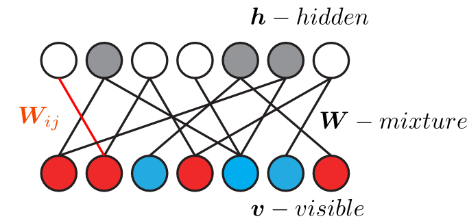 $\bm{V} = \bm{W}\bm{H}$
Independent Component Analysis
Cocktail party!
sources


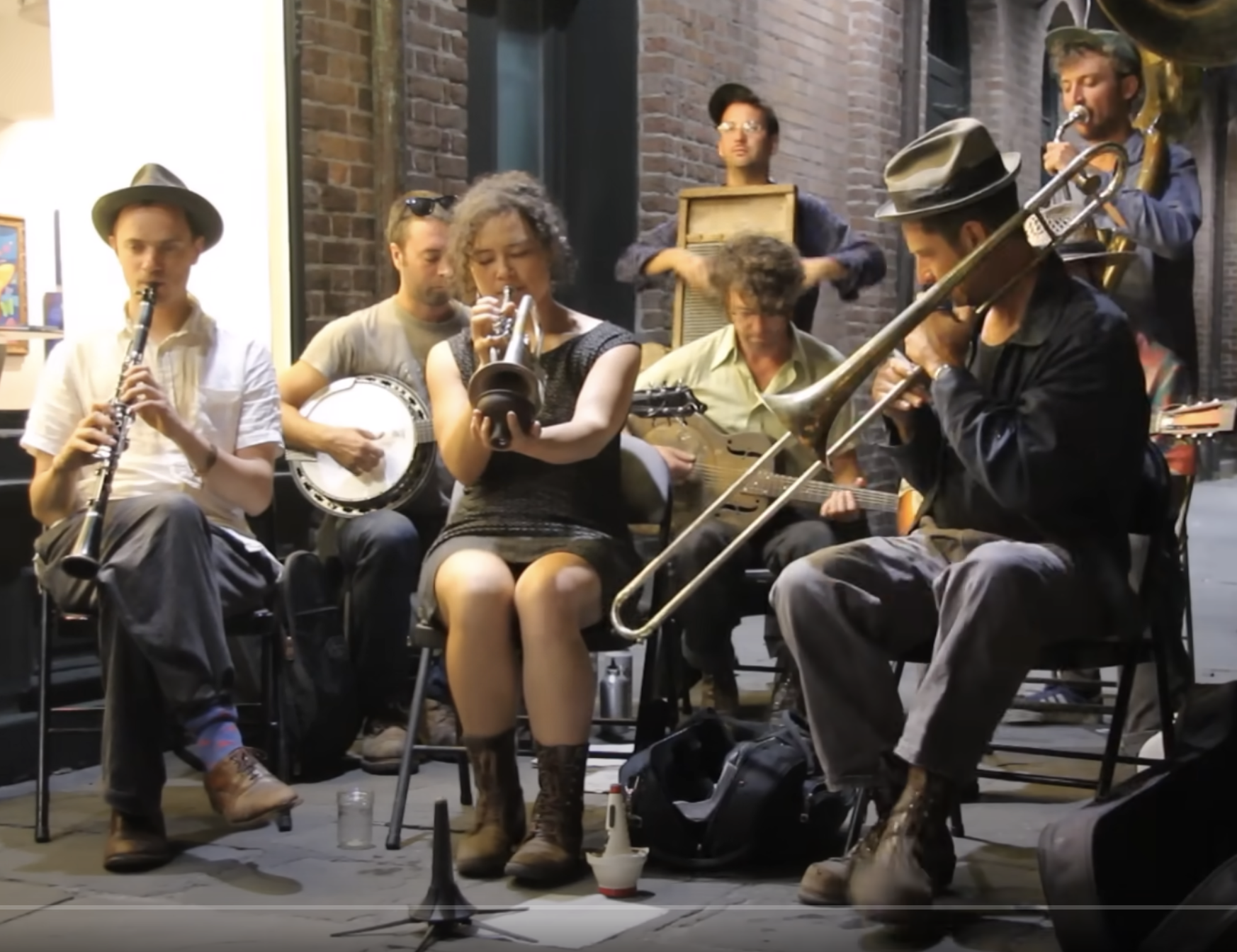
linear mixtures

reconstructions
Linear Independence
A set of vectors \(\vec{v}_1, \vec{v}_2, \dots, \vec{v}_n\) in a vector space is linearly independent if the only solution to their linear combination being zero is when all coefficients are zero.
\begin{align}
c_1 \vec{v}_1 + c_2 \vec{v}_2 + \dots + c_n \vec{v}_n = 0 \\
\implies \quad c_1 = c_2 = \dots = c_n = 0
\end{align}
Example: Vectors \((1, 0)\) and \((0, 1)\) are linearly independent.
$\vec{v}_i^T\vec{v}_j = 0$
Statistical Independence
Random variables \(X_1, X_2, \dots, X_n\) are statistically independent if the joint probability is the product of individual probabilities.
\(P(X_1, X_2) = P(X_1) \cdot P(X_2)\)
Example: The outcome of two dice rolls are independent.
Independence
Key Difference: Linear independence deals with vector spaces, while statistical independence focuses on probability distributions.
ICA: Mathematical Setup
- Given observed signals \(X\), we assume: \[ X = A \cdot S \] where \(X\) is the observed data, \(A\) is the unknown mixing matrix, and \(S\) are the independent sources.
- The goal is to recover \(S\) by finding a suitable unmixing matrix \(W\) such that: \[ Y = W \cdot X \quad \text{(where \(Y\) approximates the sources \(S\))} \]
identifiability
fastICA
Central Limit Theorem (CLT)
The Central Limit Theorem states that the sum (or average) of independent random variables with finite mean and variance tends towards a normal distribution, regardless of the original distribution.
\[
Z_n = \frac{1}{\sqrt{n}} \sum_{i=1}^n X_i \quad \xrightarrow{n \to \infty} \quad \mathcal{N}(\mu, \sigma^2)
\]
Example: The average of a large number of dice rolls will follow a normal distribution, even though a single roll is uniformly distributed.
Central Limit Theorem (CLT)
Key Insights
- Applies to independent random variables with finite mean and variance.
- Explains why sums or averages often look Gaussian, even if the original variables are not.
- The distribution converges faster with more samples.
Mathematical Implication: Mixed signals tend to be more Gaussian, which ICA exploits to recover independent, non-Gaussian sources.
CLT and Statistical Independence
The Central Limit Theorem implies that linear mixtures of independent, non-Gaussian variables tend to be more Gaussian.
\[
Z_n = \frac{1}{\sqrt{n}} \sum_{i=1}^n S_i \quad \xrightarrow{n \to \infty} \quad \mathcal{N}(\mu, \sigma^2)
\]
Key Insight: When independent sources mix linearly, the result looks more Gaussian than the original sources.
Connection between CLT and ICA
How ICA Exploits This Connection
- ICA assumes that independent sources are often non-Gaussian.
- A linear mixture (observed data) tends to be more Gaussian than the original sources.
- ICA reverses this mixing by searching for components that maximize non-Gaussianity.
Takeaway: ICA identifies independent sources by finding non-Gaussian signals within the observed mixtures, which are closer to the original, independent sources.
Nonlinear Transformations Amplify Non-Gaussianity
-
Linear transformations (e.g., rotations or scaling) preserve Gaussianity. Nonlinear transformations distort the data in ways that highlight deviations from Gaussianity.
-
Nonlinear functions like \( \tanh(u) \) or \( u^3 \) react strongly to outliers or higher-order statistics, making non-Gaussian features more prominent.
-
- Gaussian distributions have light tails—outliers are rare.
- Nonlinear functions emphasize outliers or rare events, which are common in non-Gaussian data (like sparse signals).
Nonlinear Transformations Amplify Non-Gaussianity
-
The FastICA algorithm computes expectations using these nonlinear functions, which helps it detect signals that are far from Gaussian.
-
Nonlinear transformations amplify the non-Gaussian properties in the data, making it easier to separate independent components.
FastICA: Optimization Steps
- Whiten the data: Use PCA to make the data uncorrelated. \[ Z = W_{\text{PCA}} \cdot X \]
- Choose a non-linearity (e.g., \(g(u) = \tanh(u)\)) to maximize non-Gaussianity.
- Update the weight vector \(w_i\) for each independent component: \[ w_i \leftarrow \mathbb{E} \{Z \cdot g(w_i^T Z)\} - \mathbb{E} \{g'(w_i^T Z)\} \cdot w_i \]
- Orthogonalize the weight vectors to ensure independence.
- Iterate until convergence (i.e., weight vectors stabilize).
FastICA: Implementation
import numpy as np

# Step 1: Center and whiten the data
def whiten(X):
    X = X - np.mean(X, axis=0)  # Center the data
    cov = np.cov(X, rowvar=False)  # Covariance matrix
    eigvals, eigvecs = np.linalg.eigh(cov)  # Eigen-decomposition
    D = np.diag(1.0 / np.sqrt(eigvals))  # Whitening matrix
    return X @ eigvecs @ D @ eigvecs.T

# Step 2: Nonlinear function for maximizing non-Gaussianity
def g(u):
    return np.tanh(u)  # Hyperbolic tangent nonlinearity

def g_derivative(u):
    return 1 - np.tanh(u) ** 2  # Derivative of tanh

# Step 3: FastICA iteration
def fastica(X, n_components, max_iter=100, tol=1e-5):
    X = whiten(X)
    n_samples, n_features = X.shape
    W = np.random.rand(n_components, n_features)  # Initialize random weights

    for i in range(max_iter):
        W_new = (X.T @ g(X @ W.T)) / n_samples  # Update all weights
        W_new -= np.diag(np.mean(g_derivative(X @ W.T), axis=0)) @ W_new

        # Decorrelate weights (orthogonalization)
        W_new = np.linalg.qr(W_new)[0]

        # Check for convergence
        if np.max(np.abs(np.abs(np.diag(W_new @ W.T)) - 1)) < tol:
            break
        W = W_new

    return W @ X.T  # Recovered signals

# Step 4: Example usage with synthetic data
np.random.seed(0)
S = np.array([np.sin(np.linspace(0, 8, 1000)),
              np.sign(np.sin(np.linspace(0, 8, 1000)))]).T
A = np.array([[1, 1], [0.5, 2]])  # Mixing matrix
X = S @ A.T  # Mixed signals

# Apply FastICA
S_estimated = fastica(X, n_components=2)

# Plot results
import matplotlib.pyplot as plt
fig, axs = plt.subplots(3, 1, figsize=(8, 6))
axs[0].plot(S)
axs[0].set_title('Original Signals')
axs[1].plot(X)
axs[1].set_title('Mixed Signals')
axs[2].plot(S_estimated.T)
axs[2].set_title('Recovered Signals (FastICA)')
plt.tight_layout()
plt.show()
Infomax
Infomax ICA: Maximizing Information
The Infomax principle proposes that we solve $\boldsymbol{u = Wx}$ by maximizing the information that the output $\boldsymbol{u}$ contains about the input $\boldsymbol{x}$. This is equivalent to maximizing the joint entropy $H(y)$ of a non-linearly transformed output: $$ \max_W H(y) \quad \text{where} \quad y = g(u) = g(Wx) $$
- $g(\cdot)$ is a non-linear, element-wise "squashing" function (e.g., the logistic sigmoid $\sigma(u)$).
- Maximizing the entropy of the squashed output forces the components of the linear output $\boldsymbol{u}$ to become statistically independent.
Infomax ICA: Maximizing Information
The Learning Rule
We perform gradient ascent on the objective $H(y)$. The elegant natural gradient update rule for $\boldsymbol{W}$ is:
$$ \Delta W \propto \left( I - \phi(u)u^T \right) W $$
- $I$ is the identity matrix.
- $\phi(u)$ is a non-linear "score" function derived from the probability distribution of the sources. For sources with a super-Gaussian (peaky) distribution, a common choice is $\phi(u_i) = \tanh(u_i)$.
- Intuition: This update decorrelates the outputs by adjusting $W$ to make the components of $u$ as non-Gaussian and independent as possible.
Maximal Likelihood
Nonnegative matrix factorization
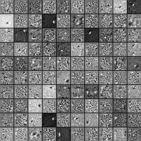
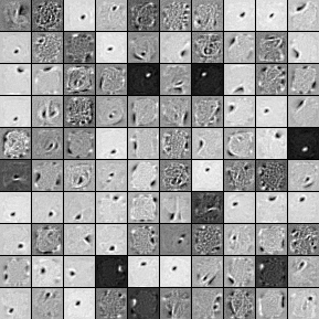
Additive features
- Features are non- negative and only add up
- Features are unknown: data comes as their combination
NMF Formally
Find a low rank non-negative approximation to a matrix
- Given data $\bm{X}$ find their factorization: \begin{align*} \bm{X} \approx \bm{W}\bm{H}\\ \bm{X}_{ij} \ge 0 \mbox{ }\bm{W}_{ij} \ge 0 \mbox{ }\bm{H}_{ij} \ge 0 \end{align*}
- Minimize the objective function: \begin{align}\nonumber E = \frac{1}{2}\|\bm{X} - \bm{W}\bm{H}\|_F^2 \end{align}
- Ignore other possible objectives
Gradient Descent
- Compute the derivative and find its zero \begin{align}\nonumber \frac{\partial E}{\partial \bm{W}} &=& \bm{WHH}^{T} - \bm{XH}^{T}\\\nonumber \frac{\partial E}{\partial \bm{H}} &=& \bm{W}^{T}\bm{WH} - \bm{W}^{T}\bm{X} \end{align}
- Classical solution \begin{align}\nonumber \bm{H} &=& \bm{H} + \bm{\eta} \odot (\bm{W}^T\bm{X} - \bm{W}^T\bm{W}\bm{H}) \end{align}
- Exponentiated gradient \begin{align}\nonumber \bm{H} &=& \bm{H}\odot e^{\bm{\eta} \odot (\bm{W}^T\bm{X} - \bm{W}^T\bm{W}\bm{H})} \end{align}
Multiplicative updates
- Setting the learning rates: \begin{align} \bm{\eta}_{\bm{H}} &= \frac{\bm{H}}{\bm{W}^T\bm{W}\bm{H}}\\ \bm{\eta}_{\bm{W}} &= \frac{\bm{W}}{\bm{W}\bm{H}\bm{H}^T}\\ \end{align}
- Results in updates: \begin{align*} \bm{H} &=& \bm{H}\odot \frac{\bm{W}^{T}\bm{X}} {\bm{W}^{T}\bm{W}\bm{H}}\\ \bm{W} &=& \bm{W}\odot \frac{\bm{X}\bm{H}^{T}} {\bm{W}\bm{H}\bm{H}^{T}} \end{align*}
Advantages:
- automatic non-negativity constraint satisfaction
- adaptive learning rate
- no parameter setting
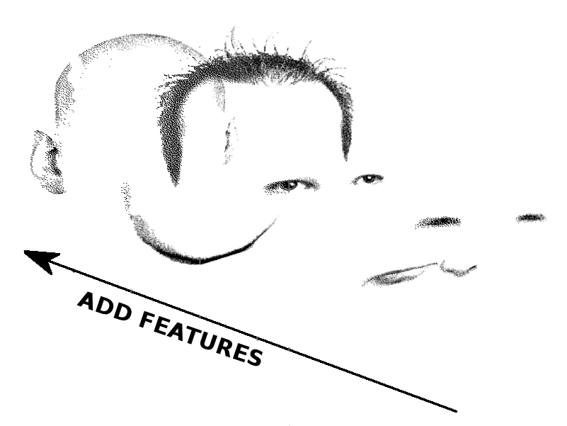
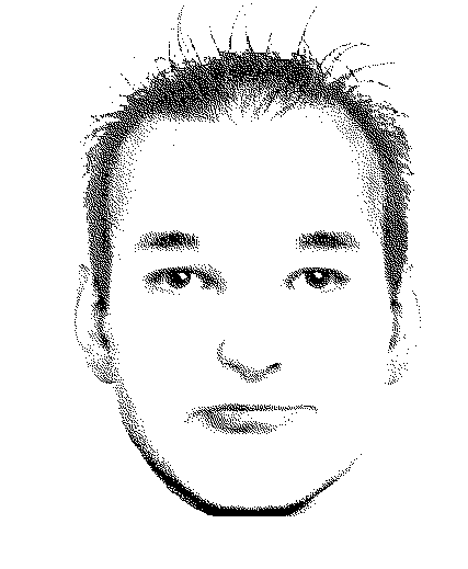
NMF on faces

NMF on hyperspectral images

Dictionary Learning
The problem
 \begin{align*}
\underset{\vec{\alpha} \in \RR^m}{\min} \frac{1}{2}\|\vec{x} - \bm{D}\vec{\alpha}\|^2_2 + \lambda\phi(\vec{\alpha})
\end{align*}
\begin{align*}
\underset{\vec{\alpha} \in \RR^m}{\min} \frac{1}{2}\|\vec{x} - \bm{D}\vec{\alpha}\|^2_2 + \lambda\phi(\vec{\alpha})
\end{align*}
Application: Denoising

Application: Compression

Autoencoders
an alternative view of PCA

Reconstruction error:
- \begin{align*} \prob{J}{\bm{X}, \bm{X}^{\prime}} & = \underset{\bm{W}}{\argmin} \|\bm{X} - \bm{X}^{\prime}\|^2 \end{align*}
- \begin{align*} \prob{J}{\bm{X}, \bm{X}^{\prime}} & = \underset{\bm{W}}{\argmin} \|\bm{X} - \bm{W}^T\bm{W}\bm{X}\|^2 \end{align*}
- Encoder \begin{align*} \bm{W} \end{align*}
- Decoder \begin{align*} \bm{W}^T \end{align*}
Even this simple model is not convex

So why limit ourselves: Autoencoder

pre-training Autoencoder

pre-training Autoencoder: MNIST
PCA vs. 784-1000-500-250-2 AE
denoising Autoencoder
Take Home Points
matrix factorization methods

Effect of sparsity parameter

Things to have in mind
Principal Component Analysis
- Finds orthogonal axes of maximal variance
- Uses full rank transform
- Can be used for compression when lower variance axes are dropped at reconstruction
- Frequently used to pre-process data
Independent Component Analysis
- A blind source separation problem
- Finds a linear transform that maximizes statistical independence of sources
- Resulting basis is not orthogonal
- Noise is often independent of the rest of data
Nonnegative Matrix Factorization
- Additive features $\to$ nonnegative problem
- Low rank approximation
- Multiplicative updates
- Nonnegativity leads to sparse solution
Dictionary Learning
- Overcomplete dictionary
- Sparse representation of samples
- Only a few bases are involved in encoding each sample
- uses explicit sparsity constraint