Advanced Machine Learning
13: Support Vector Machines
Schedule
| # | date | topic | description |
|---|---|---|---|
| 1 | 22-Aug-2022 | Introduction | |
| 2 | 24-Aug-2022 | Foundations of learning | |
| 3 | 29-Aug-2022 | PAC learnability | |
| 4 | 31-Aug-2022 | Linear algebra (recap) | hw1 released |
| 05-Sep-2022 | Holiday | ||
| 5 | 07-Sep-2022 | Linear learning models | |
| 6 | 12-Sep-2022 | Principal Component Analysis | project ideas |
| 7 | 14-Sep-2022 | Curse of Dimensionality | hw1 due |
| 8 | 19-Sep-2022 | Bayesian Decision Theory | hw2 release |
| 9 | 21-Sep-2022 | Parameter estimation: MLE | |
| 10 | 26-Sep-2022 | Parameter estimation: MAP & NB | finalize teams |
| 11 | 28-Sep-2022 | Logistic Regression | |
| 12 | 03-Oct-2022 | Kernel Density Estimation | |
| 13 | 05-Oct-2022 | Support Vector Machines | hw3, hw2 due |
| 10-Oct-2022 | * Mid-point projects checkpoint | * | |
| 12-Oct-2022 | * Midterm: Semester Midpoint | exam | |
| 14 | 17-Oct-2022 | Matrix Factorization | |
| 15 | 19-Oct-2022 | Stochastic Gradient Descent |
| # | date | topic | description |
|---|---|---|---|
| 16 | 24-Oct-2022 | k-means clustering | |
| 17 | 26-Oct-2022 | Expectation Maximization | hw4, hw3 due |
| 18 | 31-Oct-2022 | Automatic Differentiation | |
| 19 | 02-Nov-2022 | Nonlinear embedding approaches | |
| 20 | 07-Nov-2022 | Model comparison I | |
| 21 | 09-Nov-2022 | Model comparison II | hw5, hw4 due |
| 22 | 14-Nov-2022 | Model Calibration | |
| 23 | 16-Nov-2022 | Convolutional Neural Networks | |
| 21-Nov-2022 | Fall break | ||
| 23-Nov-2022 | Fall break | ||
| 24 | 28-Nov-2022 | Word Embedding | hw5 due |
| 30-Nov-2022 | Presentation and exam prep day | ||
| 02-Dec-2022 | * Project Final Presentations | * | |
| 07-Dec-2022 | * Project Final Presentations | * | |
| 12-Dec-2022 | * Final Exam | * | |
| 15-Dec-2022 | Grades due |
Outline for the lecture
- Max Margin Classifiers
- Lagrange Duality
- Dual Formulation of SVM
- Support Vector Machines
Max Margin Classifiers
bayesian decision boundary
- If $\prob{P}{\omega_1|\vec{x}} \gt \prob{P}{\omega_2|\vec{x}}$, decide $\omega_1$
- If $\prob{P}{\omega_1|\vec{x}} \lt \prob{P}{\omega_2|\vec{x}}$, decide $\omega_2$
- $\prob{P}{error|\vec{x}} = \min[\prob{P}{\omega_1|\vec{x}}, \prob{P}{\omega_2|\vec{x}}]$
Minimizing the Bayes error is the optimal strategy if we know the posterior exactly!
Decision boundary: 2 classes
In the general case, we need to non-parametrically estimate the densities
$\prob{P$_{KDE}$}{\vec{x}} = \frac{1}{Nh^d} \sum_{n=1}^N \prob{K}{\frac{\vec{x} - \vec{x}^n}{h}}$, where $\prob{K}{\vec{x}} = (2\pi)^{-d/2}e^{-\frac{1}{2}\vec{x}^T\vec{x}}$
Decision boundary is sensitive to outliers!
this derivation of SVM is due to Tong and Koller Restricted Bayes-Optimal Classifiers 2000
Restricted Bayes optimal classifier
Definition: Given a joint distribution $\prob{P$_{KDE}$}{\vec{x},C}$ and a set of classifiers $\cal H$, we say that $h^*$ is a restricted Bayes optimal classifier with respect to $\cal H$ and ${\rm P}_{KDE}$if $h^* \in {\cal H}$ and $\forall h\in {\cal H}$, $\prob{error}{h^*:{\rm P}_{KDE}} \le \prob{error}{h: {\rm P}_{KDE}}$
Restricted Decision boundary
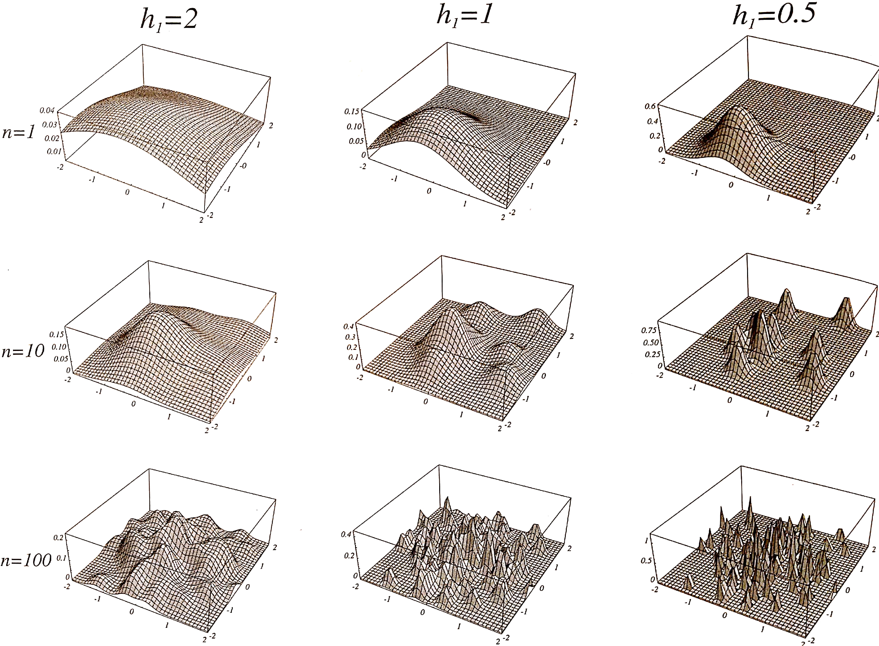
this derivation of SVM is due to Tong and Koller Restricted Bayes-Optimal Classifiers 2000
Max-margin hyperplane is Bayes optimal
this derivation of SVM is due to Tong and Koller Restricted Bayes-Optimal Classifiers 2000
Max-margin Classifier
A Hyperplane
- $r_{\color{red}{\vec{x}}} = \frac{|\vec{w}^T{\color{red} \vec{x}} + b|}{\|\vec{w}\|}$
- $r_{\color{red}{\vec{x}}} = \frac{{\color{red}{y}}(\vec{w}^T{\color{red} \vec{x}} + b)}{\|\vec{w}\|}$

DECISION "SURFACE"
$\underset{\vec{w},b}{\argmax} \{ \frac{1}{\|\vec{w}\|} \underset{i}{\min} \left[ y_i(\vec{w}^T\vec{x}_i+b)\right] \}$
w = [0.50, -0.50], b = 0.00
Min Distance: 0.00
Decision "Surface"
$\underset{\vec{w},b}{\argmax} \{ \frac{1}{\|\vec{w}\|} \underset{i}{\min} \left[ y_i(\vec{w}^T\vec{x}_i+b)\right] \}$
Observation
The distance does not depend on $\|\vec{w}\|$
- $r_i = \frac{y_i(\vec{w}^T{\vec{x}_i} + b)}{\|\vec{w}\|}$
- Scaling by $k$
- $\frac{y_i(k\vec{w}^T{\vec{x}_i} + kb)}{\|k\vec{w}\|} = \frac{k y_i(\vec{w}^T{\vec{x}_i} + b)}{k \|\vec{w}\|} = \frac{y_i(\vec{w}^T{\vec{x}_i} + b)}{\|\vec{w}\|}$
- We are free to set $y_i(\vec{w}^T{\vec{x}_i} + b)$ to whatever we want!
- Let's set it to $y_*(\vec{w}^T{\vec{x}_*} + b) = 1$ for the nearest point
Linear SVM Classifier
- The gap is distance between parallel hyperplanes \begin{align} \vec{w}^T\vec{x} + b &= -1\\ \vec{w}^T\vec{x} + b &= 1\\ \end{align}
- The gap is distance between parallel hyperplanes \begin{align} \vec{w}^T\vec{x} + (b + 1) &= 0\\ \vec{w}^T\vec{x} + (b - 1) &= 0\\ \end{align}
- $D = |b_1 - b_2|/\|\vec{w}\|$
- $D = 2/\|\vec{w}\|$
To maximize the gap, need to minimize $\|\vec{w}\|$ or equivalently $\frac{1}{2}\|\vec{w}\|^2$ ($\frac{1}{2}\vec{w}^T\vec{w}$)
Linear SVM Classifier
- Instances must be correctly classified \begin{align} \vec{w}^T\vec{x}_i + b & \le -1 \mbox{ if } y_i = -1\\ \vec{w}^T\vec{x}_i + b & \ge +1 \mbox{ if } y_i = +1\\ \end{align}
- Equivalently $y_i(\vec{w}^T\vec{x}_i + b) \ge 1$
Want to minimize $\frac{1}{2}\|\vec{w}\|^2$ subject to $y_i(\vec{w}^T\vec{x}_i + b) \ge 1$ for $i=1,\dots, N$
Classify new instance $\vec{x}$ as $f(\vec{x}) = \mbox{sign}(\vec{w}^T\vec{x} + b)$
Linear SVM: primal formulation
Minimize $\frac{1}{2}\|\vec{w}\|^2$ subject to $y_i(\vec{w}^T\vec{x}_i + b) - 1 \ge 0$ for $i=1,\dots, N$
- Primal formulation of linear SVM
- It is a convex quadratic programming (QP) optimization problem with $d$ variables and $N$ constraints
\begin{align} \underset{\vec{w} \in \RR^m}{\argmin} \vec{w}^T {\mathbf Q} \vec{w} & + \vec{w}^T\vec{c} + \epsilon \\ {\mathbf A}\vec{w} & \le \vec{b} \\ {\mathbf A} \in \RR^{n\times m}, \vec{w} & \in \RR^m, \vec{b}\in \RR^n\\ {\mathbf C}\vec{w} & = \vec{d} \\ {\mathbf C} \in \RR^{s\times m}, \vec{d} &\in \RR^s\\ \end{align}
Lagrange Duality
Joseph-Louis Lagrange
Lagrange Duality: general form
- minimize $f(x)$
- subject to
- $c_1(x) \ge 0$
- $\vdots$
- $c_C(x) \ge 0$
- $g_1(x) \le 0$
- $\vdots$
- $g_G(x) \le 0$
- $h_1(x) = 0$
- $\vdots$
- $h_H(x) = 0$
- minimize$_x$ and maximize$_{\alpha_i, \lambda_i, \mu_i}$
saddle point - \begin{align} \Lambda(x, \alpha, \lambda, \mu) & = f(x) - \sum_{i=1}^{C} \alpha_ic_i(x) \\ &+ \sum_{i=1}^{G} \lambda_i g_i(x) - \sum_{i=1}^{H} \mu_i h_i(x) \end{align}
- subject to
- $\alpha_i, \lambda_i, \mu_i \ge 0$
Necessary optimality conditions
$\frac{\partial\Lambda}{\partial x} = 0$; $\frac{\partial\Lambda}{\partial \alpha} = 0$; $\frac{\partial\Lambda}{\partial \lambda} = 0$; $\frac{\partial\Lambda}{\partial \mu} = 0$;
Karush-Kuhn-Tucker (KKT) conditions
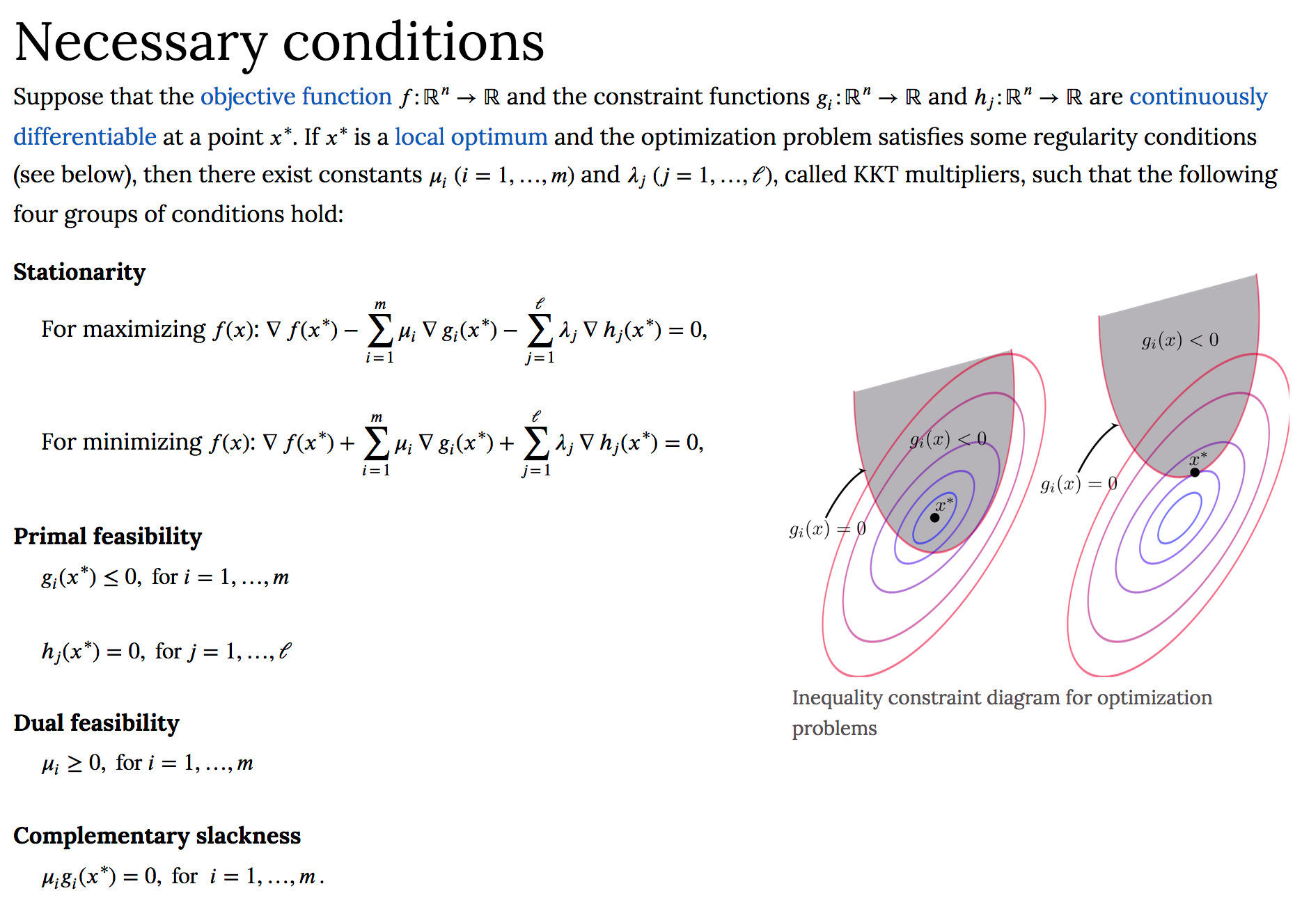
Interactive Lagrange Multipliers
surface: $z = x^2 - y^2$
constraint: $x^2 + y^2 - 1 = 0$
z value:
-0.500
Constraint Gradient ($\nabla g$)
Surface Gradient ($\nabla f$)
Lagrange Duality: example 1
$\min_x x^2$
s.t. $x \ge b$
s.t. $x\ge -1$
s.t. $x\ge 1$
Lagrange Duality: example 1
$\min_x x^2$Let's move the constraint to the objective Lagrangian
s.t. $x \ge b$ or $x-b\ge 0$
$L(x, \alpha) = x^2 - \alpha(x-b)$
s.t. $\alpha \ge 0$
Solve: $\min_x \max_{\alpha} L(x, \alpha)$
s.t. $\alpha \ge 0$
Lagrange Duality: example 1
Solve: $\min_x \max_{\alpha} L(x, \alpha)$
s.t. $\alpha \ge 0$
Lagrange Duality: example 2
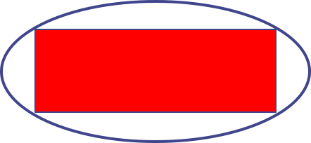
Find the largest area rectangle inside an ellipse
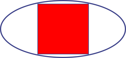
Lagrange Duality: example 2
Find the largest area rectangle inside an ellipse
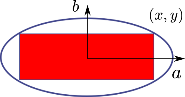
- maximize the area $4xy$
- subject to
- $\frac{x^2}{a^2} + \frac{y^2}{b^2} \le 1$
Ellipse equation
$\frac{x^2}{a^2} + \frac{y^2}{b^2} = 1$
- maximize
- $\Lambda(x,y,\alpha) = 4xy - \alpha (\frac{x^2}{a^2} + \frac{y^2}{b^2} - 1)$
- subject to
- $\alpha \ge 0$
Lagrange Duality: example 2
Find the largest area rectangle inside an ellipse
- $\frac{\partial \Lambda}{\partial x} = 4y + \frac{2\alpha x}{a^2} = 0$
- $\frac{\partial \Lambda}{\partial y} = 4x + \frac{2\alpha y}{b^2} = 0$
- $\frac{\partial \Lambda}{\partial \alpha} = \frac{x^2}{a^2} + \frac{y^2}{b^2} - 1 = 0$
- $x = \frac{a}{\sqrt{2}}$
- $y = \frac{b}{\sqrt{2}}$
- $\alpha = 2ab$
Lagrange Duality: example 2
Main point
Using Lagrangian multipliers and KKT conditions can convert a constrained problem into an unconstrained problem.
Dual formulation of SVM
Linear SVM: dual formulation
Minimize $\frac{1}{2}\|\vec{w}\|^2$ subject to $y_i(\vec{w}^T\vec{x}_i + b) - 1 \ge 0$ for $i=1,\dots, N$
- Can be recast as a "dual formulation"
- It is also a convex quadratic programming (QP) optimization problem with $N$ variables $(\alpha_i, i=1, \dots, N)$, where $N$ is the number of samples
-
Minimize $\Lambda(\vec{w}, b, \alpha) = \frac{1}{2}\|\vec{w}\|^2 - \sum_{i=1}^N \alpha_i (y_i(\vec{w}^T\vec{x}_i + b) - 1)$
-
$\frac{\partial\Lambda(\vec{w}, b, \alpha)}{\partial \vec{w}} = \vec{w} - \sum_{i=1}^N \alpha_i y_i\vec{x}_i = 0 \implies \vec{w} = \sum_{i=1}^N \alpha_i y_i \vec{x}_i$
-
Maximize $\sum_{i=1}^N \alpha_i - \frac{1}{2} \sum_{i,j=1}^N \alpha_i\alpha_j y_i y_j \vec{x}_i^T\vec{x}_j$ subject to $\alpha_i \ge 0$ and $\sum_{i=1}^N \alpha_i y_i = 0$
- Since $\vec{w} = \sum_{i=1}^N \alpha_i y_i \vec{x}_i$
- The final classifier is $f(\vec{x}) = \mbox{sign}(\sum_{i=1}^N \alpha_i y_i \vec{x}_i\vec{x} + b)$
Linear SVM: problems and solutions
The data may not be linearly separable
- $\phi(\vec{x})$: map the data into higher dimensions and hope for the best
- Soft-margin: allow some error
Support Vector Machines
Max Margin Classifiers
- Given two classes $A$ and $B$
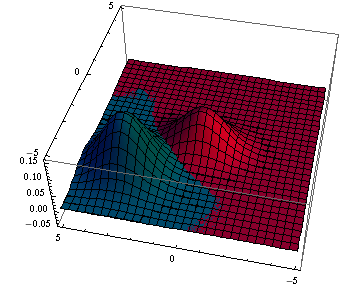
Data is a set of labeled examples $\{(\vec{x}_i,y_i)\}_{i=1}^N$ - Bayesian Decision Boundary: Distributions are known \begin{align}\nonumber g(\vec{x}) = P(A|\vec{x}) - P(B|\vec{x}) =0 \end{align}
- Maximum Margin Hyperplane: Only data is given
Mapping to Higher Dimensions
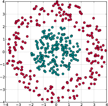
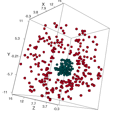
- A two class problem:
not separable by a line - Map each point into a higher dimensional space: \begin{align} \nonumber \vec{\eta}_i = \Phi(\vec{x}_i) \end{align}
- Choose $\Phi$ so the data becomes linearly separable \begin{align} \nonumber \Phi(\vec{x}) = (x_1^2,\sqrt{2}x_1x_2,x_2^2) \end{align}


Kernel Trick
Appropriate mappings are hard to construct. What to do?
- Dimensions can be many
even $\infty$ ! Have to compute very expensive inner product? - Avoid it by defining Hilbert spaces with kernels (and Mercer's theorem) \begin{align}\nonumber \langle\Phi(\vec{x}),\Phi(\vec{y})\rangle &=& \vec{k}(\vec{x},\vec{y})\\ \nonumber (x_1^2,\sqrt{2}x_1x_2,x_2^2) (y_1^2,\sqrt{2}y_1y_2,y_2^2)^T &=& (\vec{x}\cdot\vec{y})^2 \\\nonumber x_1^2y_1^2 + 2x_1x_2y_1y_2 + x_2^2y_2^2 &=& (x_1y_1 + x_2y_2)^2 \end{align}
- Take a linear algorithm, replace inner products with kernels and get a nonlinear algorithm as a result!

Kernel Trick for SVM
Maximize $\sum_{i=1}^N \alpha_i - \frac{1}{2} \sum_{i,j=1}^N \alpha_i\alpha_j y_i y_j \vec{x}_i^T\vec{x}_j$
subject to $\alpha_i \ge 0$ and $\sum_{i=1}^N \alpha_i y_i = 0$
The final classifier is $f(\vec{x}) = \mbox{sign}(\sum_{i=1}^N \alpha_i y_i \vec{x}_i\vec{x} + b)$
Maximize $\sum_{i=1}^N \alpha_i - \frac{1}{2} \sum_{i,j=1}^N \alpha_i\alpha_j y_i y_j K(\vec{x}_i,\vec{x}_j)$
subject to $\alpha_i \ge 0$ and $\sum_{i=1}^N \alpha_i y_i = 0$
The final classifier is $f(\vec{x}) = \mbox{sign}(\sum_{i=1}^N \alpha_i y_i K(\vec{x}_i, \vec{x}) + b)$
Maximize $\vec{\alpha}^T\vec{1} - \frac{1}{2} \vec{\alpha}^T\vec{y}^T{\bm G}\vec{y} \vec{\alpha}$
subject to $\vec{\alpha} \ge 0$ and $\vec{\alpha}^T \vec{y} = 0$
Mercer's theorem
$K(\vec{x}, \vec{y})$ is a kernel function iff it is symmetric (i.e. $K(\vec{x}, \vec{y}) = K(\vec{y}, \vec{x})$) and positive semidefinite (i.e. $\vec{x}^T{\bm G}\vec{x} \ge 0, \forall \vec{x} \in \RR^n$)
Creating kernels is an art but some generative rules can help
- An inner product is a kernel $K(\vec{x},\vec{y}) = \vec{x}^T\vec{y}$
- A constant is a kernel $K(\vec{x},\vec{y}) = 1$
- Kernel product is a kernel $K(\vec{x},\vec{y}) = K_1(\vec{x},\vec{y})K_2(\vec{x},\vec{y})$
- $\forall \psi: X \to \RR$ product of $\psi$ is a kernel $K(\vec{x},\vec{y}) = \psi(\vec{x})\psi(\vec{y})$
- Nonnegatively weighted linear combination of kernels is a kernel $K(\vec{x},\vec{y}) = \alpha_1K_1(\vec{x},\vec{y}) + \alpha_2K_2(\vec{x},\vec{y}), {\rm s.t. } \alpha_i \ge 0$
- and a few more
Kernels do not guarantee linear separabillity
Soft Margin SVM
Let's introduce slack variables $\xi_i \ge 0$ allowing mistakes
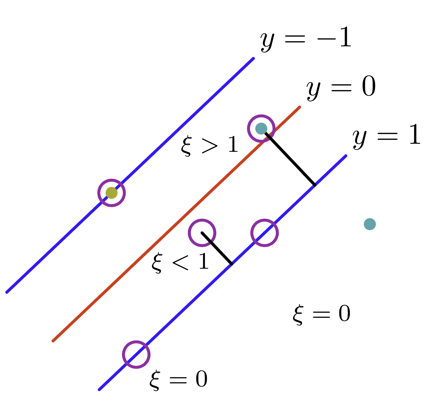
Maximize $\vec{\alpha}^T\vec{1} - \frac{1}{2} \vec{\alpha}^T\vec{y}^T{\bm G}\vec{y} \vec{\alpha}$
subject to $C \ge \vec{\alpha} \ge 0$ and $\vec{\alpha}^T \vec{y} = 0$
Soft Margin SVM
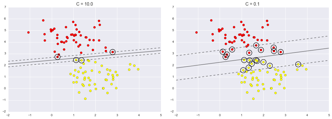
Changing the constraints: $y_i(\vec{w}^T\vec{x} + b) \ge 1 - \xi_i$
Modifies the primal problem: $C\sum_{i=1}^N \xi_i + \frac{1}{2}\|\vec{w}\|^2$
Take home points
Advantages
- Quadratic programming with a single optimum (efficient)
- Sparse solutions based on supports
- Great generalization thanks to the max margin!
Disadvantages
- Sensitive to noise and outliers in data
- Making or choosing kernel for the task is an art
- Dependence on soft-margin hyperparameter
Reading References
- Books:
- Bishop - Chapt. 7 (pg. 325-360)
- Shai - Chapt. 15 (pg. 201-220)
- SVM Notes
- Kernel Methods paper
