Advanced Machine Learning

12: Kernel Density Estimation

Schedule (you are here )

Outline of this lecture

• Non-parametric Density Estimation & Histograms
• Parzen Windows & Kernel Density Estimation
• Bandwidth Selection & Bias-Variance Tradeoff
• Multivariate Density Estimation & Pre-whitening
• Non-parametric Classification & Bridge to SVM
• Take Home Points

Connecting the Dots: The Road to Non-parametric Methods

Non-parametric Density Estimation

bayesian decision boundary

• If $\prob{P}{\omega_1|\vec{x}} \gt \prob{P}{\omega_2|\vec{x}}$, decide $\omega_1$
• If $\prob{P}{\omega_1|\vec{x}} \lt \prob{P}{\omega_2|\vec{x}}$, decide $\omega_2$
• $\prob{P}{error|\vec{x}} = \min[\prob{P}{\omega_1|\vec{x}}, \prob{P}{\omega_2|\vec{x}}]$
• $\prob{P}{\omega_1|\vec{x}} = \prob{P}{\omega_2|\vec{x}}$ decision boundary
• $\log\frac{\prob{P}{\omega_1|\vec{x}}}{\prob{P}{\omega_2|\vec{x}}} = 0$

Non-parametric density estimation

We have assumed that either

• The likelihoods $\prob{P}{\vec{x}|\omega_k}$ were known (likelihood ratio test), or
• At least their parametric form was known (parameter estimation)

Ooh! How challenging exciting!

Histogram

• Divide the sample space into a number of bins;
• Approximate the density by the fraction of training data points that fall into each bin

  $$\prob{P}{\vec{x}} = \frac{1}{N}\frac{\text{# of } \vec{x}^i \text{ in the same bin as }\vec{x}}{\text{bin width}}$$

• Need to define: bin width and first bin starting position
• 

Histogram is simple but problematic

• The density estimate depends on the starting bin position
• The discontinuities of the estimate are only an artifact of the chosen bin locations
• The curse of dimensionality, since the number of bins grows exponentially with the number of dimensions
• Unsuitable for most practical applications except for quick visualizations in one or two dimensions
• Let's leave it alone!

Interactive: Histogram Sensitivity & Artifacts

Non-parametric DE

general formulation

What we are trying to accomplish?

• The probability that $\vec{x}\sim \prob{P}{\vec{x}}$, will fall in a given region $\cal R$ of the sample space is \[ \theta = \int_{\cal R} \prob{P}{\vec{x}^{\prime}}d\vec{x}^{\prime} \]
• Probability that $k$ of $N$ drawn vectors $\{\vec{x}^1, \dots, \vec{x}^N\}$ will fall in region ${\cal R}$ is \[ \prob{P}{k} = {N \choose k} \theta^k (1 - \theta)^{N-k} \]
• From properties of the binomial pmf $\prob{E}{\frac{k}{N}} = \theta$ $\prob{var}{\frac{k}{N}} = \frac{\theta(1-\theta)}{N}$
• As $N\rightarrow\infty$, variance reduces and we can obtain a good estimate from $ \theta \simeq \frac{k}{N} $

Non-parametric DE

general formulation

• Assume $\cal R$ is so small that $\prob{P}{\vec{x}}$ does not much vary across it \[ \theta = \int_{\cal R} \prob{P}{\vec{x}^{\prime}}d\vec{x}^{\prime} \simeq \prob{P}{\vec{x}}V \]
• Combining with $\theta \simeq \frac{k}{N}$ \[ \prob{P}{x} \simeq \frac{k}{NV} \]

• We obtain a more accurate estimate increasing $N$ and shrinking $V$

practical considerations

• As $V$ approaches zero ${\cal R}$ encloses no examples
• Have to find a compromise for $V$
• The general expression of nonparametric density becomes

  \[ \prob{P}{x} \simeq \frac{k/N}{V} \mbox{, where } \begin{cases} V & \text{volume surrounding } \vec{x} \\ N & \text{total #examples}\\ k & \text{#examples inside } V \end{cases} \]

• For convergence of the estimator we need to provide for:

  \begin{align} &\underset{n\to\infty}{\lim} V = 0\\ &\underset{n\to\infty}{\lim} k = \infty\\ &\underset{n\to\infty}{\lim} k/N = 0\\ \end{align}

Two approaches that provide this

• Fix $V$ and estimate $k$ - kernel density estimation (KDE)
• Fix $k$ and estimate $V$ - k-nearest neighbor (kNN)

Parzen Windows & KDE

Parzen windows

• Assume the region $\cal R$ enclosing $k$ examples is a hypercube with side of length $h$ centered at $\vec{x}$
• Its volume is $V = h^d$, where $d$ is the dimensionality
• To find the number of examples that fall within this region we define a window function $K(u)$ (a.k.a. kernel) \[ \prob{K}{u} = \begin{cases} 1 & |u_j| \lt \frac{1}{2} \forall j = 1\dots d\\ 0 & \text{otherwise} \end{cases} \]
• Known as a Parzen window or the naïve estimator and corresponds to a unit hypercube centered at the origin
• $\prob{K}{\frac{(\vec{x} - \vec{x}^n)}{h}} = 1$ if $\vec{x}^n$ is inside a hypercube of side $h$ centered on $\vec{x}$, and zero otherwise

Parzen windows

• The total number of points inside the hypercube is \[ k = \sum_{n=1}^N \prob{K}{\frac{\vec{x} - \vec{x}^n}{h}} \]
• The density estimate becomes \[ \prob{P$_{KDE}$}{\vec{x}} = \frac{1}{Nh^d} \sum_{n=1}^N \prob{K}{\frac{\vec{x} - \vec{x}^n}{h}} \]

Note: Parzen window resembles a histogram, but with the window locations determined directly by the data!

Parzen windows

• What's the role of the kernel function?
• Let us compute the expectation of the estimate $\prob{P$_{KDE}$}{\vec{x}}$ \begin{align} E\left[\prob{P$_{KDE}$}{\vec{x}}\right] &= \frac{1}{Nh^d} \sum_{n=1}^N E\left[\prob{K}{\frac{\vec{x} - \vec{x}^n}{h}}\right]\\ & = \frac{1}{h^d} E\left[ \prob{K}{\frac{x-x^\prime}{h}}\right]\\ & = \frac{1}{h^d} \int \prob{K}{\frac{x-x^\prime}{h}} \prob{P}{x^\prime}dx^\prime\\ \end{align}
• $\prob{P$_{KDE}$}{\vec{x}}$ is a convolution of the true density with the kernel function!
• As $h\to 0$, the kernel approaches the Dirac delta and $\prob{P$_{KDE}$}{\vec{x}}$ approaches true density

Exercise

• Given dataset $X = \{4, 5, 5, 6, 12, 14, 15, 15, 16, 17\}$ use Parzen windows to estimate the density at $y=3,10,15$; use $h=4$
• 
• Let's estimate $\prob{P}{y=3}$: $$ \frac{1}{10\times 4^1} \left[ \prob{K}{\frac{3-4}{4}} + \prob{K}{\frac{3-5}{4}} + \cdots +\prob{K}{\frac{3-17}{4}}\right] = \frac{1}{40} = 0.025 $$
• $ \prob{P}{y=10} = \frac{1}{10\times 4^1} \left[ 0 + 0 + 0 + 0 + 0 + 0 + 0 + 0 + 0 + 0\right] = \frac{0}{40} = 0 $
• $ \prob{P}{y=15} = \frac{1}{10\times 4^1} \left[ 0 + 0 + 0 + 0 + 0 + 1 + 1 + 1 + 1 + 0\right] = \frac{4}{40} = 0.1 $

Interactive: Parzen Window (Box Kernel) Accumulator

Smooth kernels

• The Cube window has a few drawbacks
  • Yields density estimates that have discontinuities
  • Weights equally all points $\vec{x}_i$, regardless of their distance to the estimation point $\vec{x}$
• Often a smooth kernel is preferred
  • $\prob{K}{\vec{x}} \ge 0$
  • $\displaystyle\int_{\cal R} \prob{K}{\vec{x}}d\vec{x} = 1$
  • Usually radially symmetric and unimodal, e.g. $\prob{K}{\vec{x}} = (2\pi)^{-d/2}e^{-\frac{1}{2}\vec{x}^T\vec{x}}$
• Just use it in our density estimator: $$ \prob{P$_{KDE}$}{\vec{x}} = \frac{1}{Nh^d} \sum_{n=1}^N \prob{K}{\frac{\vec{x} - \vec{x}^n}{h}} $$

Interpretation

• The smooth kernel estimate is a sum of "bumps"
• The kernel function determines the shape of the bumps
• The parameter $h$, "smoothing parameter" determines their width
• 

Interactive: Smooth KDE & The "Sum of Bumps"

Bandwidth Selection

Prior knowledge vs data

bandwidth selection

• Large $h$ over-smoothes the DE hiding structure
• Small $h$ yields a spiky uninterpretable DE

bandwidth selection

• Pick $h$ that minimizes the error between the estimated density and the true density
• Let us use MSE for measuring this error
• $E\left[ (\prob{P$_{KDE}$}{\vec{x}} - \prob{P}{\vec{x}})^2 \right] $
• $ = E\left[ \prob{P$_{KDE}$}{\vec{x}}^2 - 2 \prob{P$_{KDE}$}{\vec{x}} \prob{P}{\vec{x}} + \prob{P}{\vec{x}}^2\right]$
• $ = E\left[ \prob{P$_{KDE}$}{\vec{x}}^2\right] - 2 E\left[\prob{P$_{KDE}$}{\vec{x}}\right] \prob{P}{\vec{x}} + \prob{P}{\vec{x}}^2$
• Add and subtract $E^2\left[ \prob{P$_{KDE}$}{\vec{x}} \right]$
• \begin{align} = & E^2\left[ \prob{P$_{KDE}$}{\vec{x}} \right] - 2 E\left[\prob{P$_{KDE}$}{\vec{x}}\right] \prob{P}{\vec{x}} + \prob{P}{\vec{x}}^2 \\ & + E\left[ \prob{P$_{KDE}$}{\vec{x}}^2\right] - E^2\left[ \prob{P$_{KDE}$}{\vec{x}} \right] \end{align}
• \begin{align} = & (E\left[ \prob{P$_{KDE}$}{\vec{x}} \right] - \prob{P}{\vec{x}})^2 + E\left[ \prob{P$_{KDE}$}{\vec{x}}^2\right] - E^2\left[ \prob{P$_{KDE}$}{\vec{x}} \right] \end{align}
• This is an exact example of the bias-variance tradeoff: $$ \text{MSE}(h) = \text{Bias}^2(h) + \text{Variance}(h) $$

Bias-variance tradeoff (digression)

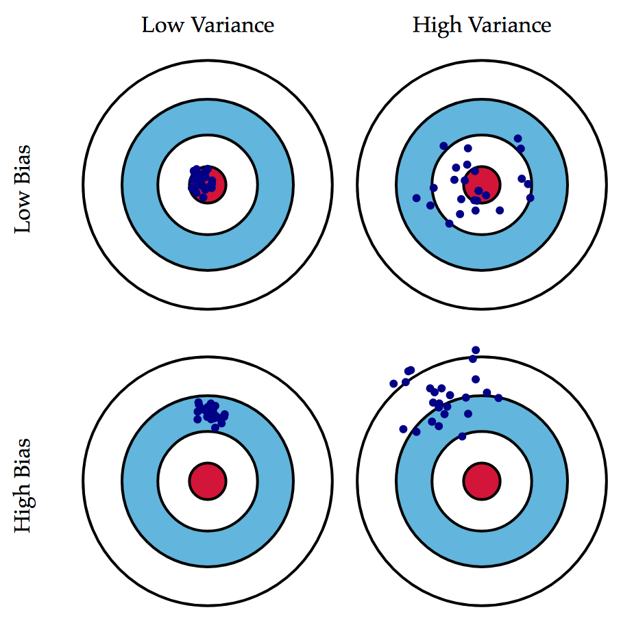
Bias-variance tradeoff (digression)

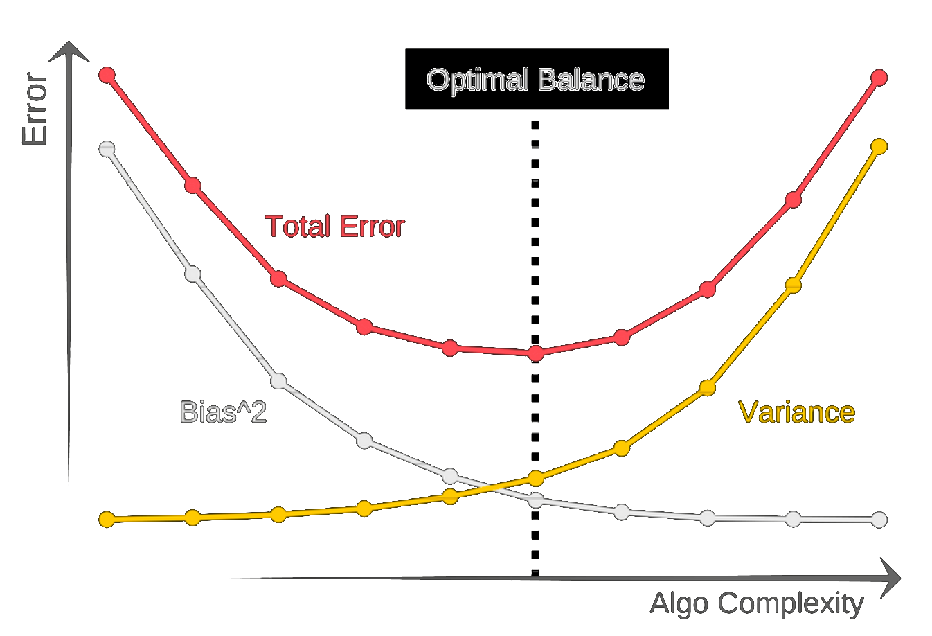
Bias-variance tradeoff (digression)

bandwidth selection

• Plot out several curves and choose the estimate that best matches your subjective ideas
• Not too practical for high-dimensional data

• Minimize the overall MSE $ h = \argmin \{ E\left[ \int (\prob{P$_{KDE}$}{\vec{x}} - \prob{P}{\vec{x}})^2 d\vec{x} \right]\} $
• Assuming the true distribution is Gaussian: $ h^* = 1.06\sigma N^{-\frac{1}{5}} $
• Can obtain better results with: $$ h^* = 0.9A N^{-\frac{1}{5}} \mbox{ where } A = \min(\sigma, \frac{IQR}{1.34}) $$

Interactive: Bias-Variance Tradeoff & Silverman's Rule

Unimodal distribution KDE

• 100 data points were drawn from the distribution
• True density (left), the estimates using $h=1.06\sigma N^{-1/5}$ (middle) and $h=0.9A N^{-1/5}$ (right)

bimodal distribution KDE

• 100 data points were drawn from the distribution
• True density (left), the estimates using $h=1.06\sigma N^{-1/5}$ (middle) and $h=0.9A N^{-1/5}$ (right)

Multivariate KDE

Multivariate density estimation

• $h$ is the same for all the axes, so this density estimate is weighting all axes equally
• A problem if one or several of the features has larger spread than the others

• Pre-scaling each axis (e.g. to unit variance)
• Pre-whitening the data
  • Whiten the data $\vec{y}=\Lambda^{-1/2}V^T\vec{x}$
  • Estimate the density
  • Transform everything back
  • Equivalent to hyper-ellipsoidal kernel

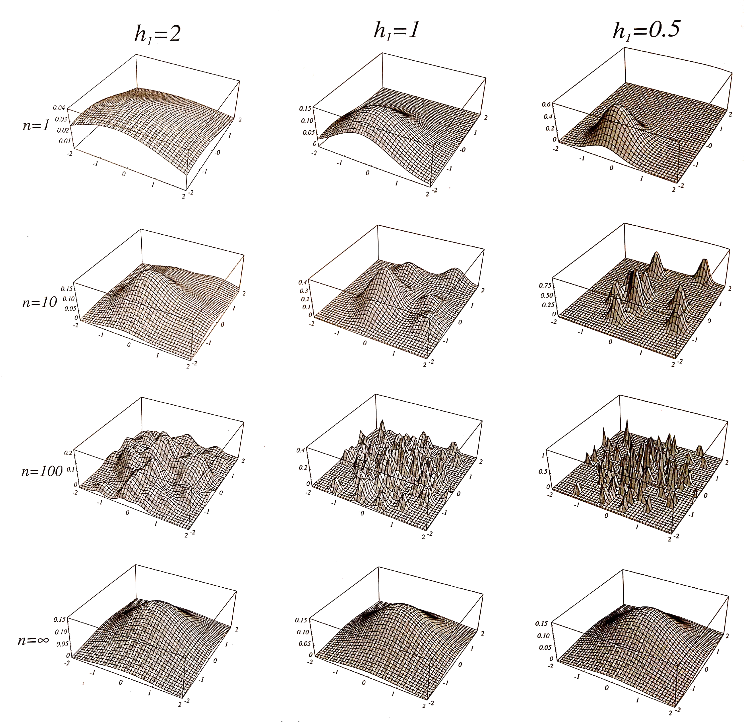
Product kernels

• $\prob{P$_{KDE}$}{\vec{x}} = \frac{1}{N} \sum_{i=1}^N \prob{K}{\vec{x}, \vec{x}^i, h_1, \dots, h_d}$
• $\prob{K}{\vec{x}, \vec{x}^i, h_1, \dots, h_d} = \frac{1}{h_1h_2\dots h_d} \prod_{j=1}^d \prob{K}{\frac{x_j-x_j^i}{h_j}} $
• Consists of the product of one-dimensional kernels
• Note, kernel independence does not imply feature independence!

Interactive: 2D Multivariate KDE & Anisotropy

Non-parametric Classification

The Dual: $k$-Nearest Neighbors

• In KDE, we fixed $V = h^d$ and estimated $k$ (count inside fixed volume)
• In $k$-NN, we fix $k$ and let the volume $V(\vec{x})$ adapt: $$ \prob{P$_{k\text{NN}}$}{\vec{x}} = \frac{k}{N \cdot V(\vec{x})} = \frac{k}{N \cdot V_d \cdot r_k^d(\vec{x})} $$ where $r_k(\vec{x})$ is the Euclidean distance to the $k$-th nearest neighbor of $\vec{x}$, and $V_d$ is the volume of the unit sphere in $\mathbb{R}^d$.
• Local Adaptive Resolution:
  • Dense regions $\implies$ small $r_k(\vec{x})$, tiny $V(\vec{x})$ $\implies$ high spatial resolution
  • Sparse regions $\implies$ large $r_k(\vec{x})$, large $V(\vec{x})$ $\implies$ heavy smoothing

$k$-NN Classification as Bayes Decision

• Unconditional density estimate: $\prob{P}{\vec{x}} = \frac{k}{N V}$
• Class-conditional likelihood: $\prob{P}{\vec{x}|\omega_i} = \frac{k_i}{N_i V}$
• Class prior probability: $\prob{P}{\omega_i} = \frac{N_i}{N}$
• Plugging into Bayes' Rule: $$ \prob{P}{\omega_i|\vec{x}} = \frac{\prob{P}{\vec{x}|\omega_i}\prob{P}{\omega_i}}{\prob{P}{\vec{x}}} = \frac{\left(\frac{k_i}{N_i V}\right) \left(\frac{N_i}{N}\right)}{\frac{k}{N V}} = \mathbf{\frac{k_i}{k}} $$

• The intuitive $k$-NN majority vote is the exact Bayes posterior under $k$-NN density estimation!

Decision boundary: 2 classes

In the general case, we estimate class densities non-parametrically using KDE:

$\prob{P$_{KDE}$}{\vec{x}|\omega} = \frac{1}{Nh^d} \sum_{n=1}^N \prob{K}{\frac{\vec{x} - \vec{x}^n}{h}}$, where $\prob{K}{\vec{x}} = (2\pi)^{-d/2}e^{-\frac{1}{2}\vec{x}^T\vec{x}}$

Warning: The non-parametric decision boundary is highly sensitive to outliers!

Interactive: 2-Class KDE Boundary & Outlier Vulnerability

Restricted Bayes Optimal Classifier

The Dilemma: Non-parametric KDE boundaries have high variance and are sensitive to outliers. As $h \to 0$, the estimate degenerates into delta spikes at each point.

Tong & Koller (AAAI 2000):
To control variance, restrict the hypothesis class $\mathcal{H}$ to linear hyperplanes.

Next Lecture:
The max-margin hyperplane is the Restricted Bayes-Optimal Classifier!

→ Support Vector Machines (SVM)

Take Home Points

• Beyond Parametric Forms: Estimate $p(\vec{x})$ directly from empirical data without assuming fixed distribution families.
• Parzen Windows: Eliminate rigid histogram bins by centering smooth kernels at each data point.
• Bandwidth Controls Bias-Variance: Kernel shape matters little; bandwidth $h$ governs overfitting vs. oversmoothing ($h^* \propto N^{-1/5}$).
• Multivariate Scaling: Isotropic kernels fail under correlated features; resolve with pre-whitening or product kernels.
• Duality & Bridge to SVMs: $k$-NN adapts volume for fixed $k$; KDE boundary sensitivity motivates max-margin hyperplanes.