Advanced Machine Learning

11: Logistic Regression

Schedule (you are here )

#	date	topic	description
1	24-Aug-2026	Introduction
2	26-Aug-2026	Foundations of learning	Drop/Add
3	31-Aug-2026	PAC learnability	HW1
4	02-Sep-2026	Linear learning models
5	07-Sep-2026	Labor Day Holiday	Holiday
6	09-Sep-2026	Principal Component Analysis	Project ideas
7	14-Sep-2026	Curse of Dimensionality	HW2, HW1 due
8	16-Sep-2026	Bayesian Decision Theory
9	21-Sep-2026	Parameter estimation: MLE
10	23-Sep-2026	Parameter estimation: MAP & NB	finalize teams
11	28-Sep-2026	Logistic Regression	HW3, HW2 due
12	30-Sep-2026	Kernel Density Estimation
13	05-Oct-2026	Support Vector Machines
14	07-Oct-2026	Matrix Factorization
15	12-Oct-2026	* Midterm	Exam, HW3 due
16	14-Oct-2026	k-means clustering
17	19-Oct-2026	Invited: Intro to Causal Learning I

#	date	topic	description
18	21-Oct-2026	Invited: Intro to Causal Learning II
19	26-Oct-2026	* Mid-point projects checkpoint	HW4, P
20	28-Oct-2026	Expectation Maximization
21	02-Nov-2026	Stochastic Gradient Descent
22	04-Nov-2026	Automatic Differentiation
23	09-Nov-2026	Nonlinear embedding approaches	HW5, HW4 due
24	11-Nov-2026	Model comparison
25	16-Nov-2026	Model Calibration
26	18-Nov-2026	Convolutional Neural Networks
27	23-Nov-2026	Thanksgiving Break	Holiday
28	25-Nov-2026	Thanksgiving Break	Holiday
29	30-Nov-2026	Word Embedding
30	02-Dec-2026	Project Final Presentations	HW5 due, P
31	07-Dec-2026	Presentation spillover / Exam prep	Classes End
32	09-Dec-2026	* Final Exam	Exam
33	16-Dec-2026	Project Reports	due
34	17-Dec-2026	Grades due 5 p.m.	PAWS

Outline of this lecture

Naïve Bayes recap: Probabilistic Linear Boundaries
Defining Logistic Regression & Geometry
The GNB – Logistic Regression Connection
Solving Logistic Regression (MLE & IRLS)
Take Home Points

Naïve Bayes (recap)

Properties and assumptions

Features $X_i$ and $X_j$ are conditionally independent given the class label $Y$

$\prob{P}{X_i,X_j|Y} = \prob{P}{X_i|Y}\prob{P}{X_j|Y}$

$\prob{P}{X_1,\dots, X_d|Y} = \prod_{i=1}^d \prob{P}{X_i|Y}$

$f_{NB}(\vec{x}) = \underset{y}{\argmax} \prod_{i=1}^d \prob{P}{x_i|y}\prob{P}{y}$

Assume a parametric form for $\prob{P}{X_j|Y}$ and $\prob{P}{Y}$

Estimate MLE parameters for these functions.
Plug in and operate the NB classifier

Gaussian Naïve Bayes

$Y \sim \mbox{Bernoulli}(\pi)$ $\prob{P}{X_i = \vec{x}_i|Y = y_k} = \frac{1}{\sigma_{ik}\sqrt{2\pi}} e^{-\frac{(\vec{x}_i - \mu_{ik})^2}{2\sigma_{ik}^2}}$

Different mean and variance for each class $k$ and each pixel $i$.$^*$

Let's assume variance is independent of class: $\sigma_{ik} = \sigma_{i}$

Gaussian NB as a linear classifier

$\prob{P}{X_i = \vec{x}_i|Y = y_k} = \frac{1}{\sigma_{ik}\sqrt{2\pi}} e^{-\frac{(\vec{x}_i - \mu_{ik})^2}{2\sigma_{ik}^2}}$

For simplicity consider 2 class problem $\sigma_{i,0} = \sigma_{i, 1}$
Decision boundary:
$\prod_{i=1}^d \prob{P}{x_i|y=0}\prob{P}{y=0} = \prod_{i=1}^d \prob{P}{x_i|y=1}\prob{P}{y=1}$
Equivalently:
$\log\frac{\prod_{i=1}^d \prob{P}{x_i|y=0}\prob{P}{y=0}}{\prod_{i=1}^d \prob{P}{x_i|y=1}\prob{P}{y=1}} = 0$ $\log\frac{\prod_{i=1}^d \prob{P}{x_i|y=0}\prob{P}{y=0}}{\prod_{i=1}^d \prob{P}{x_i|y=1}\prob{P}{y=1}}= \log\frac{1 - \pi}{\pi} +\sum_{i=1}^d \log\frac{\prob{P}{x_i|y=0}}{\prob{P}{x_i|y=1}}$

Gaussian NB as a linear classifier

Condition: Equal Feature Variance Across Classes ($\sigma_{i,0}^2 = \sigma_{i,1}^2 = \sigma_i^2$)

Decision boundary ($\log\text{-odds} = 0$):
$\log\frac{\prod_{i=1}^d \prob{P}{x_i|y=0}\prob{P}{y=0}}{\prod_{i=1}^d \prob{P}{x_i|y=1}\prob{P}{y=1}} = 0 \implies \log\frac{1 - \pi}{\pi} +\sum_{i=1}^d \log\frac{\prob{P}{x_i|y=0}}{\prob{P}{x_i|y=1}} = 0$
When variances are equal, quadratic $x_i^2$ terms cancel:
$\log\frac{1 - \pi}{\pi} +\sum_{i=1}^d \frac{\mu^2_{i,1} - \mu^2_{i,0}}{2\sigma_i^2} + \sum_{i=1}^d \frac{\mu_{i,1} - \mu_{i,0}}{\sigma_i^2} x_i = w_0 + \sum_{i=1}^d w_i x_i = 0$
A Probabilistic Linear Boundary: $w_0 + \vec{w}^T\vec{x} = 0$
(If class variances differ $\sigma_{i,0}^2 \ne \sigma_{i,1}^2$, quadratic terms survive $\implies$ curved boundary: Quadratic Discriminant Analysis / QDA).

Key conceptual point: a linear decision boundary can be obtained probabilistically! Earlier in the course, we studied the Perceptron, which is a purely algorithmic linear classifier that updates its hyperplane on misclassified points. Here, Gaussian Naïve Bayes demonstrates that a strictly linear decision boundary ($w_0 + \vec{w}^T\vec{x} = 0$) also emerges purely probabilistically from Gaussian class-conditional distributions when classes share feature variance. Notice: 1. Shared variance (\sigma_{i,0} = \sigma_{i,1}) across classes cancels the quadratic x_i^2 terms. If variances differ, the boundary curves into Quadratic Discriminant Analysis (QDA). 2. Unequal priors \pi \ne 0.5 only shift the scalar intercept w0 parallelly without bending the line.

Generative vs. Discriminative

Generative classifiers (such as Naïve Bayes)
- Assume a functional form for $\prob{P}{x,y}$ (or $\prob{P}{x|y}$ and $\prob{P}{y}$)
- Estimate parameters of $\prob{P}{x|y}$ and $\prob{P}{y}$ from training data
- Able to generate samples from a trained model
Note:
$\underset{y}{\argmax} \prob{P}{x|y}\prob{P}{y} = \underset{y}{\argmax} \prob{P}{y|x}$
Let's learn $\prob{P}{y|x}$ directly!
Or learn the decision boundary directly

Defining Logistic regression

And the winner is...

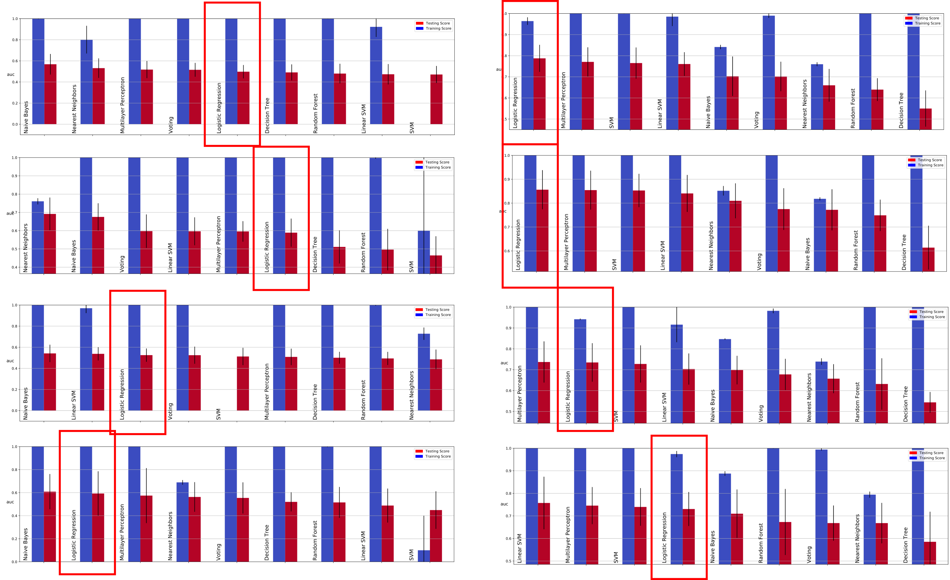
Example

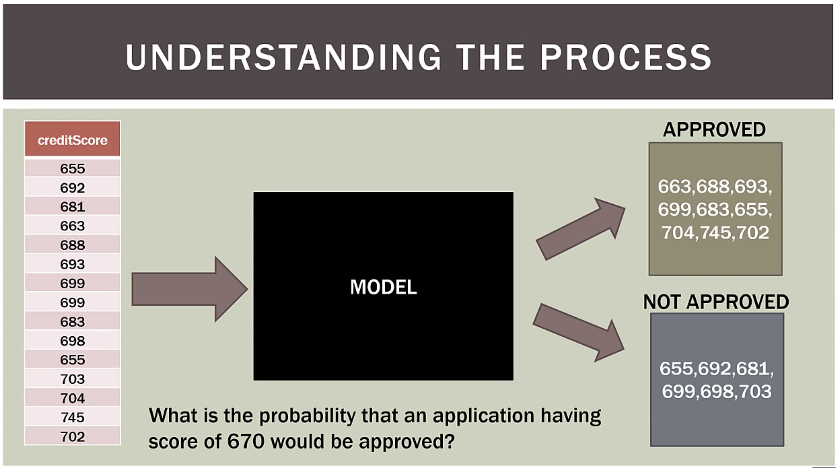
Problem definition

Logistic regression seeks to

Model the probability of an event occuring depending on the values of the independent variables, which can be categorical or numerical
Estimate the probability that an event occurs for a randomly selected observation versus the probability that the event does not occur
Predict the effect of a series of variables on a binary response variable
Classify observations by estimating the probability that an observation is in a particular category (e.g. approved or not approved for a loan)

Our data in 1D: Why Not Linear Regression?

Bounding Probabilities & Robustness to Outliers

Linear OLS: -- Logistic Reg: --

Scenarios:

Outlier Position x: 7.5

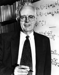
Sir David Cox

Why not SVM?

Odds

Probability	Corresponding odds
0.5	50:50 or 1
0.9	90:10 or 9
0.999	999:1 or 999
0.01	1:99 or 0.0101
0.001	1:999 or 0.001001

Log-Odds

Log-odds	Probability
0	0.5
2.19	0.9
6.9	0.999
-4.6	0.01
-6.9	0.001

Linear Fit to Log-Odds

\begin{array}{ll} \log\left(\frac{p_+}{1-p_+}\right) &= kx + b\\ &= w_1 x + w_0 \\ &= \vec{w}^T\vec{x} \\ \end{array}

\begin{array}{ll} \log\left(\frac{\prob{P}{G=1|X=x}}{\prob{P}{G=K|X=x}}\right) &= \vec{w}_1^T\vec{x}\\ \log\left(\frac{\prob{P}{G=2|X=x}}{\prob{P}{G=K|X=x}}\right) &= \vec{w}_2^T\vec{x}\\ &\vdots \\ \log\left(\frac{\prob{P}{G=K-1|X=x}}{\prob{P}{G=K|X=x}}\right) &= \vec{w}_{K-1}^T\vec{x}\\ \end{array}

What's the probability?

$\log\left(\frac{p_+}{1-p_+}\right) = \vec{w}^T\vec{x}$
$\frac{p_+}{1-p_+} = e^{\vec{w}^T\vec{x}}$
$p_+ = e^{\vec{w}^T\vec{x}}(1-p_+)$
$p_+ = e^{\vec{w}^T\vec{x}}-p_+e^{\vec{w}^T\vec{x}}$
$p_++p_+e^{\vec{w}^T\vec{x}} = e^{\vec{w}^T\vec{x}}$
$p_+(1+e^{\vec{w}^T\vec{x}}) = e^{\vec{w}^T\vec{x}}$
$p_+ = \frac{e^{\vec{w}^T\vec{x}}}{1+e^{\vec{w}^T\vec{x}}}$
$p_+ = \frac{1}{1+e^{-\vec{w}^T\vec{x}}}$

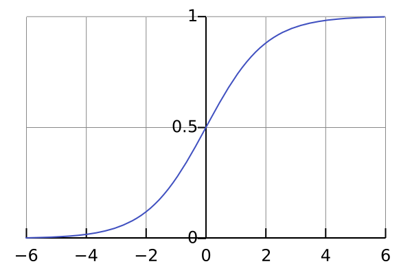
Geometry of Logistic Regression

Decision Boundary (Hyperplane in ℝ^d) vs. Probability Output (Nonlinear Sigmoid Surface)

                          Boundary: wᵀx + w₀ = 0  |  Surface: P(Y=1|x) = σ(wᵀx + w₀)
                        

Level Set P=0.5: Hyperplane | Surface: Sigmoid Ramp

Presets:

Orientation θ: Bias w₀:

Let's address the fundamental geometric nature of Logistic Regression: 1. Is Logistic Regression a linear or nonlinear classifier? It is STRICTLY a linear classifier! The decision boundary where P(Y=1|x) = 0.5 is defined by w^T x + w0 = 0. In 2D, this is a straight line; in d dimensions, it is a flat linear hyperplane. 2. However, the probability output P(Y=1|x) = sigma(w^T x + w0) is a nonlinear sigmoidal surface (shown in 3D on the right). It squashes the real line to (0, 1), producing an S-shaped ramp perpendicular to the hyperplane boundary. 3. Notice that all parallel contour lines in feature space are linear hyperplanes. The normal vector w determines the orientation and steepness of the ramp, while w0 shifts the hyperplane across feature space without rotating it. Drag the 3D perspective to see how the flat hyperplane level set cuts through the middle (p=0.5) of the sigmoidal ramp.

What's the probability when it is interesting?

$\prob{P}{G=k|X=x} = \frac{e^{\vec{w}_k^T\vec{x}}}{1+\sum_i^{K-1}e^{\vec{w}_i^T\vec{x}}}, k = 1, \dots, K-1$
$\prob{P}{G=K|X=x} = \frac{1}{1+\sum_i^{K-1}e^{\vec{w}_i^T\vec{x}}}$

Softmax!

\[ \sigma(\mathbf{z})_i = \frac{e^{z_i}}{\sum_{j=1}^K e^{z_j}} \]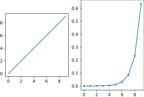 linear softmax

Interactive Softmax & Temperature

$\sigma(\mathbf{z})_i = \frac{e^{z_i / T}}{\sum_{j=1}^K e^{z_j / T}}$ — Multi-Sample Segmentation & Temperature Filtering

                          Sample: Sample 1 (#720)
                          Temp T: 1.00
                          Peak: #720
                          Max P: --
                          Entropy: --
                        

Samples:

Softmax acts as a smooth, differentiable approximation of the argmax operator. In this demo, we explore multi-sample segmentation across 1000 logit channels: • Click S1, S2, S3 to cycle through three different sample inputs (with signal peaks at channels #720, #525, and #950, matching the original slide SVGs). Notice how the softmax distribution shifts its focus dynamically to isolate the dominant channel for each sample! • Try "Rivals" to see what happens when two rival channels have nearly identical logits (#310 and #680). At T=1.0, they split the probability mass (~45% each). Lowering T to 0.15 forces softmax to decisively pick the winner, while raising T blends them into the uniform background noise. • This temperature-scaled softmax is exactly how Transformers and LLMs perform token sampling and attention segmentation.

Gaussian NB implies Logistic Sigmoid!

Equal Class Variances ($\sigma_{i,0}^2 = \sigma_{i,1}^2$) $\implies$ Linear Log-Odds $\implies$ Sigmoid Posterior

Recall: in Gaussian NB with equal variances, log-odds is linear:
$\log\frac{\prob{P}{Y=1|\vec{x}}}{\prob{P}{Y=0|\vec{x}}} = w_0 + \sum_{i=1}^d w_i x_i = w_0 + \vec{w}^T\vec{x}$
Inverting log-odds yields the exact same Logistic Sigmoid:
$\prob{P}{Y=1|\vec{x}} = \frac{1}{1 + \exp(-(w_0 + \vec{w}^T\vec{x}))} = \sigma(w_0 + \vec{w}^T\vec{x})$
Equal Variance Condition: Quadratic $x_i^2$ terms cancel only when classes share feature variance ($\sigma_{i,0}^2 = \sigma_{i,1}^2$). If class variances differ, the boundary curves (Quadratic Discriminant Analysis / QDA).
(Note: Unequal priors $\pi \ne 0.5$ only shift the scalar intercept $w_0$ parallelly, keeping the boundary linear).

GNB vs. Logistic Regression

Generative (Diagonal Covariance) vs. Discriminative (Direct Boundary)

True Density GNB Model GNB: -- LR: --

Presets:

Feature Correlation ρ: 0.75

An alternative perspective on log odds

What's posterior probability of class $c_1$ given a sample $\vec{x}$?

\[ \prob{p}{c_1|\vec{x}} = \frac{\prob{p}{\vec{x}|c_1}\prob{p}{c_1}}{\prob{p}{\vec{x}|c_1}\prob{p}{c_1} + \prob{p}{\vec{x}|c_2}\prob{p}{c_2}} \]

Let's introduce $a = \ln\frac{\prob{p}{\vec{x}|c_1}\prob{p}{c_1}}{\prob{p}{\vec{x}|c_2}\prob{p}{c_2}}$

\[ \prob{p}{c_1|\vec{x}} = \frac{1}{1+\exp{(-a)}} = \sigma(a) \]

Logistic Sigmoid

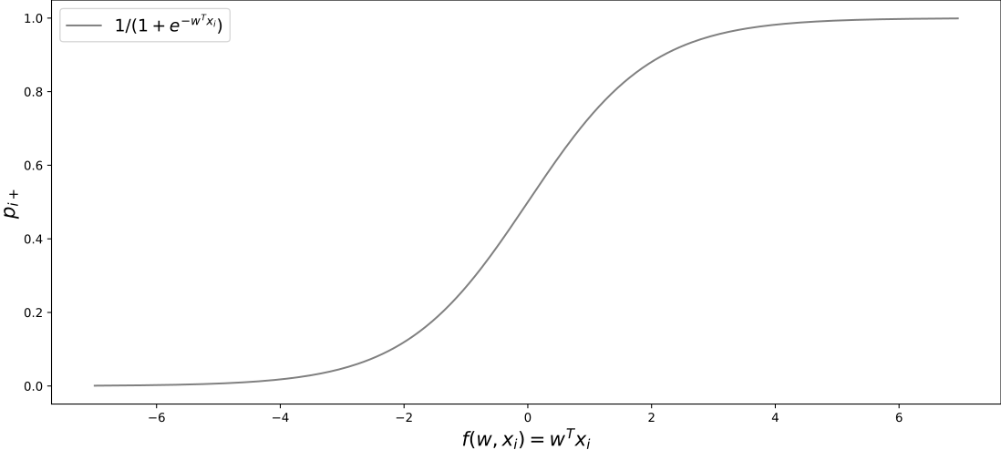
Nice properties of logistic sigmoid \begin{align} \sigma{(-a)} &= 1 - \sigma{(a)}\\ \end{align} $a = \ln{(\frac{\sigma}{1 - \sigma})} \color{#dc322f}{\text{ log odds???}}$
$\frac{d\sigma}{d a} =\sigma(1-\sigma)$

Solving Logistic regression

Maximum likelihood estimate

\begin{align} {\cal l}(\vec{w}) &= \underset{\vec{w}}{\argmax} \prod_i^N P_{\vec{w}}(c_k | x_i)\\ {\cal l}(\vec{w}) &= \underset{\vec{w}}{\argmax} \prod_{i:\vec{x}_i \in c_1}^N P_{\vec{w}}(c_1 | x_i)\prod_{i:\vec{x}_i \in c_2}^N P_{\vec{w}}(c_2 | x_i)\\ {\cal l}(\vec{w}) &= \underset{\vec{w}}{\argmax} \prod_{i:\vec{x}_i \in c_1}^N \sigma \prod_{i:\vec{x}_i \in c_2}^N (1 - \sigma)\\ {\cal l}(\vec{w}) &= \underset{\vec{w}}{\argmax} \prod_i^N \sigma_i^{l_1}(1 - \sigma_i)^{1-l_1}\\ \end{align}

Negative Log likelihood

\begin{align} {\cal l}(\vec{w}) &= \underset{\vec{w}}{\argmax} \prod_i^N \sigma_i^{l_1}(1 - \sigma_i)^{1-l_1}\\ \ell(\vec{w}) &= - \sum_i^N ({l_i}\ln(\sigma_i) + (1-l_i)\ln(1 - \sigma_i))\\ \end{align}

Cross Entropy (recap)

\[ H_{p,q} = -\sum_{i=1}^n p_X(x_i) \log q_X(x_i) \]

Negative Log likelihood: How to solve for $\vec{w}$?

\begin{align} \ell(\vec{w}) &= - \sum_i^N ({l_i}\ln(\sigma_i) + (1-l_i)\ln(1 - \sigma_i))\\ \nabla_{\vec{w}} \ell &= \sum_i^N (\sigma_i - l_i)\vec{x}_i\\ \nabla_{\vec{w}} \ell &= {\bf X}^T (\vec{\sigma} - \vec{l}) \stackrel{\text{set}}{=} 0\\ \end{align}

Taylor expansion

\[ f(x) = f(a)+\frac {f^\prime(a)}{1!} (x-a)+ \frac{f''(a)}{2!} (x-a)^2+ \cdots \] \[ f(x) = \sum_{n=0} ^ {\infty} \frac {f^{(n)}(a)}{n!} (x-a)^{n} \]

Interactive Taylor Expansion

From Tangent Slopes (Gradient Descent) to Osculating Parabolas (Newton-Raphson)

                          T₂(x) = f(a) + f'(a)(x-a) + ½ f''(a)(x-a)²
                        

Function:

Order n:

Center a: 0.50

Newton-Raphson method

\begin{align} \ell(\vec{w} + \Delta) & = \ell(\vec{w}) + \ell^{\prime}(\vec{w})\Delta + \frac{1}{2}\ell^{\prime\prime}(\vec{w})\Delta^2\\ \frac{\partial \ell(\vec{w} + \Delta)}{\partial \Delta} & \stackrel{set}{=} 0 \\ \ell^{\prime}(\vec{w}) + \ell^{\prime\prime}(\vec{w})\Delta &= 0\\ \Delta &= - \frac{\ell^{\prime}(\vec{w})}{\ell^{\prime\prime}(\vec{w})}\\ \vec{w}_{new} & = \vec{w}_{old} + \Delta = \vec{w}_{old}- \frac{\ell^{\prime}(\vec{w})}{\ell^{\prime\prime}(\vec{w})}\\ \vec{w}_{new} & = \vec{w}_{old} - {\bf H}^{-1}\nabla_\vec{w}\ell \end{align}

Hessian

\[ \mathbf H = \begin{bmatrix} \dfrac{\partial^2 f}{\partial w_1^2} & \dfrac{\partial^2 f}{\partial w_1\,\partial w_2} & \cdots & \dfrac{\partial^2 f}{\partial w_1\,\partial w_n} \\[2.2ex] \dfrac{\partial^2 f}{\partial w_2\,\partial w_1} & \dfrac{\partial^2 f}{\partial w_2^2} & \cdots & \dfrac{\partial^2 f}{\partial w_2\,\partial w_n} \\[2.2ex] \vdots & \vdots & \ddots & \vdots \\[2.2ex] \dfrac{\partial^2 f}{\partial w_n\,\partial w_1} & \dfrac{\partial^2 f}{\partial w_n\,\partial w_2} & \cdots & \dfrac{\partial^2 f}{\partial w_n^2} \end{bmatrix} \]

Newton-Raphson update for linear regression

$f(\vec{w}) = \sum_{i}^{n} (\vec{w}^T\vec{x}_i - y_i)^2$

Let us write in matrix form:
$f(\vec{w}) = (\bf{X}\vec{w} - \vec{y})^T(\bf{X}\vec{w} - \vec{y})$

The gradient:
$\nabla_\vec{w}f = \bf{X}^T\bf{X}\vec{w} - \bf{X}^T\vec{y}$

The Hessian:
$\nabla^2_\vec{w}f = \bf{X}^T\bf{X}$

$\vec{w}_{new} = \vec{w}_{old} - (\bf{X}^T\bf{X})^{-1}(\bf{X}^T\bf{X}\vec{w}_{old} - \bf{X}^T\vec{y})$

$\vec{w}_{new} = \vec{w}_{old} - \vec{w}_{old} + (\bf{X}^T\bf{X})^{-1}\bf{X}^T\vec{y}$

$\vec{w}_{new} = (\bf{X}^T\bf{X})^{-1}\bf{X}^T\vec{y}$

Newton-Raphson update for logistic regression

IRLS: Iteratively Reweighted Least Squares

$\nabla_{\vec{w}} \ell = {\bf X}^T (\vec{\sigma} - \vec{l})$
${\bf H} = \nabla\nabla_{\vec{w}} \ell = {\bf X}^T{\bf W}{\bf X}$
${\bf W}_{i,i} = \sigma_i(1-\sigma_i)$
$\vec{w}_{new} = \vec{w}_{old} - (\bf{X}^T\bf{W}\bf{X})^{-1}\bf{X}^T(\vec{\sigma} - \vec{l})$
bring $(\bf{X}^T\bf{W}\bf{X})^{-1}$ out
$\vec{w}_{new} = (\bf{X}^T\bf{W}\bf{X})^{-1}(\bf{X}^T\bf{W}\bf{X}\vec{w}_{old} - \bf{X}^T(\vec{\sigma} - \vec{l}))$
$\vec{z} = \bf{X}\vec{w}_{old} - \bf{W}^{-1}(\vec{\sigma} - \vec{l})$ (adjusted response)
$\vec{w}_{new} = (\bf{X}^T\bf{W}\bf{X})^{-1}\bf{X}^T\bf{W}\vec{z}$ ← Weighted Least Squares form

Why IRLS? Because weights ${\bf W}_{i,i} = \sigma_i(1-\sigma_i)$ depend on $\vec{w}$, we solve weighted least squares repeatedly with recomputed weights until convergence.

Take Home Points

Generative vs. Discriminative Bridge: Gaussian NB with equal class variance implies the logistic sigmoid $P(Y=1|X) = \sigma(\vec{w}^T\vec{x})$; Logistic Regression retains this form while dropping normality and feature independence assumptions.
Linear Classifier, Nonlinear Probability Surface: The decision boundary $\vec{w}^T\vec{x} + w_0 = 0$ is strictly a flat linear hyperplane in feature space $\mathbb{R}^d$, while the predicted posterior $P(Y=1|\vec{x}) = \sigma(\vec{w}^T\vec{x} + w_0)$ is a bounded nonlinear sigmoidal surface.
Convexity & Cross-Entropy: Logistic negative log-likelihood is strictly convex with no local minima; its gradient $\mathbf{X}^T(\vec{\sigma} - \vec{y})$ reflects prediction errors weighted by inputs.
Second-Order Optimization (IRLS): Newton-Raphson approximates the loss via its 2nd-order Taylor expansion; the update $\vec{w}_{\text{new}} = (\mathbf{X}^T\mathbf{W}\mathbf{X})^{-1}\mathbf{X}^T\mathbf{W}\vec{z}$ solves iteratively reweighted least squares with Hessian curvature $\mathbf{X}^T\mathbf{W}\mathbf{X}$.
Multiclass Softmax & Temperature: Softmax generalizes logistic regression to $K$ classes; temperature scaling smoothly interpolates between uniform distribution ($T \to \infty$) and hard argmax ($T \to 0$).